![]()
![]()
![]()
Use LEFT and RIGHT arrow keys to navigate between flashcards;
Use UP and DOWN arrow keys to flip the card;
H to show hint;
A reads text to speech;
602 Cards in this Set
- Front
- Back
|
Week 01 Dependence |
A condition in which two random variables are not independent. X and Y are positively dependent if the conditional probability, P(X|Y), of X given Y is greater than the probability of X, P(X), or equivalently if P(X&Y) > P(X)*P(Y). They are negatively dependent if the inequalities are reversed. Notice that in what I see as an extreme case to help illustrate this example the p(x) or p(y) or both could be zero in which case if (x&y) is not null or empty, it will be greater than zero the result of p(x)*p (y). Now that if x and y are disjoint (mutually exclusive) then the p(x&y) is zero. Therefore conditional probability does not include sets that are disjoint.
Examples: The probability of a union (marriage) vs. finding a single person
Or natural occurring elements in combination vs. individual components. |
|
|
Week 02 Independence |
Two processes are INDEPENDENT if knowing the outcome of one event provides no useful information about the outcome of the other event.
P(A|B) = P(A), then A and B are independent. In other words, B has no likelihood on the outcome of A |
|
|
Week 02 Complement |
The sum of all variables are equal to 1 but cannot be greater than 1 |
|
|
Week 01 Union |
The joining of two sets to make one set where repeated (overlapping) elements are included only once.
The Venn Diagram is a good visual example. Union is considered disjoining and is called a disjunction where the components are disjuncts. |
|
|
Week 01 Law of Large Numbers |
In probability theory, the law of large numbers (LLN) is a theorem that describes the result of performing the same experiment a large number of times. According to the law, the average of the results obtained from a large number of trials should be close to the expected value, and will tend to become closer as more trials are performed. |
|
|
Week 01 p-value |
P(observed OR more extreme outcome | HsubKnot is true).
The probability of obtaining a test statistic result at least as extreme or as close to the one that was actually observed, assuming that the null hypothesis is true. Another way of saying this, is the p-value is the probability of observing data at least as favorable to the alternative hypothesis as our current data set, if the null hypothesis is true P(e|h), where e is the observed data, event or evidence and h is the hypothesis. We typically use a summary statistic, in some cases the mean, to help compute the p-value, by finding the summary statistic's z-score, and evaluate the hypothesis. (See pg. 179 OpenIntro Statistics for and example of a z-score and corresponding p-value.)
A researcher will often "reject the null hypothesis" when the p-value turns out to be less than a predetermined significance level, often 0.05[3][4] or 0.01. Such a result indicates that the observed result would be highly unlikely under the null hypothesis. |
|
|
Week 01 Boxplot |
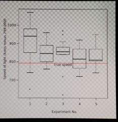
In descriptive statistics, a box plot or boxplot is a convenient way of graphically depicting groups of numerical data through their quartiles. This is a good way of showing categorical to numerical variables. Box plots may also have lines extending vertically from the boxes (whiskers) indicating variability outside the upper and lower quartiles, hence the terms box-and-whisker plot and box-and-whisker diagram. Outliers may be plotted as individual points.
Box and whisker plots are uniform in their use of the box: the bottom and top of the box are always the first and third quartiles, and the band inside the box is always the second quartile (the median). But the ends of the whiskers can represent several possible alternative values, among them: * the minimum and maximum of all of the data[1] (as in Figure 2) |
|
|
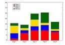
Week 01 Barplot |
|
|
|
Week 01 Histogram |
![In statistics, a histogram is a graphical representation of the distribution of data. It is an estimate of the probability distribution of a continuous variable and was first introduced by Karl Pearson.[1] A histogram is a representatio...](https://images.cram.com/images/upload-flashcards/80/16/89/6801689_m.png)
In statistics, a histogram is a graphical representation of the distribution of data. It is an estimate of the probability distribution of a continuous variable and was first introduced by Karl Pearson.[1]
A histogram is a representation of tabulated frequencies, shown as adjacent rectangles or squares (in some situations), erected over discrete intervals (bins), with an area proportional to the frequency of the observations in the interval. The height of a rectangle is also equal to the frequency density of the interval, i.e., the frequency divided by the width of the interval.
The total area of the histogram is equal to the number of data. A histogram may also be normalized displaying relative frequencies. It then shows the proportion of cases that fall into each of several categories, with the total area equaling 1.
The categories are usually specified as consecutive, non-overlapping intervals of a variable. The categories (intervals) must be adjacent, and often are chosen to be of the same size.[2] The rectangles of a histogram are drawn so that they touch each other to indicate that the original variable is continuous. |
|
|
Week 01 Normal Probability Plot |
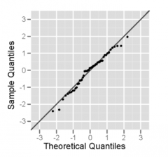
The normal probability plot is a graphical technique to identify substantive departures from normality. This includes identifying outliers, skewness, kurtosis, a need for transformations, and mixtures. Normal probability plots are made of
In a normal probability plot (also called a "normal plot"), the sorted data are plotted vs. values selected to make the resulting image look close to a straight line if the data are approximately normally distributed. Deviations from a straight line suggest departures from normality. The plotting can be manually performed by using a special graph paper, called normal probability paper. With modern computers normal plots are commonly made with software.
The normal probability plot is a SECIAL CASE of the Q–Q probability plot for a normal distribution. The theoretical quantiles are generally chosen to approximate either the mean or the median of the corresponding order statistics. |
|
|
Week 01 Mosaic plot |
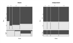
The categorical variables are first put in order. Then each variable is assigned to an axis. In the table on the right, sequence and classification is given for the example. Another order or assignment will result in a different mosaic plot, i.e., as in all multivariate plots, the order of variables plays a role. At the left edge of the first variable "Gender" is plotted. All of the data are first divided into two blocks: The strip includes, among all females, the upper, larger block all male. One sees immediately that much less (about one quarter) of the people on the ship were female. At the top of the second variable "Class" is applied. The four vertical columns are therefore for the four values of these variables (1st, 2nd, 3rd, and crew). These columns are not the same width. The width of a column indicates the relative frequency of this occurrence again. One can see that for men, the crew represents the largest group among women in the third class passengers were the largest group. There were only a few women crew. The third variable "Survived" is shown on the right side and also highlighted by the color: The dark gray rectangles represent the people who did not survive the disaster. One sees immediately that the women in the first class had the best chances of survival. In general, the probability was the misfortune to survive higher for women than for men and for 1st class passenger higher than for the other passengers. Overall, about 1/3 of all people survived (light gray areas). |
|
|
Week 01 Theorem |
As a mnemonic, the T stands for truth. Logically, many theorems are of the form of an indicative conditional: if A, then B. Such a theorem does not assert B, only that B is a necessary consequence of A. In this case A is called the hypothesis of the theorem (note that "hypothesis" here is something very different from a conjecture) and B the conclusion (formally, A and B are termed the antecedent and consequent). |
|
|
Week 01 Hypothesis |
A
made on the basis of limited evidence as a starting point for further investigation. |
|
|
Week 01 Supposition |
An uncertain belief. |
|
|
Week 01 Null hypothesis |
The status quo, that is, the hypothesis that there is no significant difference between specified populations, any observed difference being due to sampling or experimental error.
There is nothing going on, leaves everything up to chance and there is independence.
|
|
|
Week 01 Inference |
A conclusion reached on the basis of evidence and reasoning. It follows a hypothesis. |
|
|
Week 01 Alternative Hypothesis |
In statistical hypothesis testing, the alternative hypothesis (or maintained hypothesis or research hypothesis) and the null hypothesis are the two rival hypotheses which are compared by a statistical hypothesis test.
The alternative hypothesis represents our research question. |
|
|
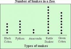
Week 01 Dot plot |
|
|
|
Week 01 How does one conduct a hypothesis test? |
Assume the null hypothesis is true and the observe the effects. If the effects are what is supposed to happen then the hypothesis is true UNDER THE CONDITIONS (IN OTHER WORDS, GIVEN) |
|
|
Week 01 What is 68%, 95% and 99.7%? |
The probability that the observation is respectively within 1,2 or 3 standard deviations of the mean. |
|
|
Week 01 Explain the relationship between pnorm and qnorm in R. |
They are inverse functions.
pnorm(z) is pnorm of z where z is the z score and returns the area to the LEFT of the Z score or the probability
qnorm(p) is qnorm of p where p is the probaility (area) whose upper bound is contained by the z-score (number of standard deviations) returned (yielded) by qnorm.
In mathematics, an inverse function is a function that "reverses" another function: if the function f applied to an input x gives a result of y, then applying its inverse function g to y gives the result x, and vice versa. i.e., f(x) = y if and only if g(y) = x. A function f that has an inverse is said to be invertible. When it exists, the inverse function is uniquely determined by f and is denoted by f −1, read f inverse. Superscripted "−1" does not, in general, refer to numerical exponentiation. In some situations, for instance when f is an invertible real-valued function of a real variable, the relationship between f and f−1 can be written more compactly, in this case, f−1(f(x)) = x = f(f−1(x)), meaning f−1 composed with f, in either order, is the identity function on R. |
|
|
Week 01 Describe the z-score table in detail. |
The most left or right column represents the z-score (or standard deviation) to the tenths place. the remaining columns represent the z-score to the hundreds or two-digits place. The center of the table represents probabilities (percentiles or areas). |
|
|
Week 01 What is a z-score and what is the equation to calculate it? |
A z-score is a statistical measurement of a score's relationship to the mean in a group of scores. A z-score of 0 means the score is the same as the mean. A z-score can also be positive or negative, indicating whether it is above or below the mean and by how many standard deviations.
z = (x-mu)/std
x - observation mu - population mean std - standard deviation |
|
|
Week 01 What is the relationship between the functions pnorm() and qnorm()? |
qnorm() returns the standard deviation (aka z-score) and pnorm() is probability that an event or occurence is within z standard deviations of the mean and is calculated by computing the the area under the curve left of the z-score (or standard deviation), both apply to normal distributions. |
|
|
Week 01 What are the three ways to calculate the area under the curve (probability)? |
Calculator on the web, saved in favorites |
|
|
Week 03 When does one reject the null hypothesis? |
If the evidence is overwhelming for the alternative hypothesis. The p-value is less than the significance level. Conceptually, when the event is extreme assuming the hypothesis is true then one would reject the null hypothesis. |
|
|
Week 03 When does one reject the alternative hypothesis? |
If the evidence is overwhelming for the null hypothesis. if p-value is > significance level. |
|
|
Week 03 How does one do hypothesis testing (for a single mean)? |
Set the Hypothesis HsubKnot : mu = null value, Set HsubA mu <, > or not equal to null value. |
|
|
Week 03 What is a point estimate and what is the point estimate representation for the mean? |
It is an estimate (sample statistic) of a population parameter using data from the sample. The point estimate representation for the mean is x bar. |
|
|
Week 03 How does one find the critical value (z*), z star? |
If the confidence interval is 95% then find the area not contained by the interval, that is 5% (.05) and divide by 2.
Take the result .025 and find it in
|
|
|
Week 03 What is the difference between the confidence level and the confidence interval? |
The confidence level is expressed as a percent of confidence that the point estimate is within the margin of error of the population parameter.
For example, a 95% confidence level would mean that a sample taken would put the point estimate within x bar + or - margin of error 95% of the time where the margin of error is z* (derived from the confidence level) times the standard error, where standard error is the stddev of the sample, a placeholder for the stddev of the population, divided by the square of the number of samples. this makes sense since the more samples one takes the margin of error will get smaller. The confidence level is defined by a range that contains the point estimate at the confidence level.
|
|
|
Should one ever base the hypothesis on the sample statistics (e.g. x bar) as opposed to mu? |
No. It makes sense that the sample statistics cannot be generalized to the population as a whole. However, they can be used to test a hypothesis based on parameters of the population. |
|
|
Week 01 How does one represent the confidence interval? |
General confidence for any case is a point estimate +- margin of error. This example applies to a z distribution.
where z* is selected to correspond to the confidence level, and SE represents the standard error.
The value z*SE is called the margin of error. |
|
|
Week 02 Mutually Exclusive |
Disjoint ( as heads and tails are in a coin ), that is, they can not occur at the same time. Complements are disjoint and, therefore, mutually exclusive. |
|
|
Central Limit Theorem (CLT) |
In probability theory, the central limit theorem (CLT) states that, GIVEN CERTAIN CONDITIONS, the arithmetic mean of a sufficiently large number of iterates of independent random variables, each with a well-defined expected value and well-defined variance, WILL BE APPROXIMATELY normally distributed. Conditions: The Central Limit Theorem states that whenever a random sample of size n is taken from any distribution with mean µ and variance r^2, then the sample mean will be approximately normally distributed with mean µ and variance r^2. The larger the value of the sample size n, the better the approximation to the normal. This is because the tests use the sample mean , which the Central Limit Theorem tells us will be approximately normally distributed. |
|
|
Sampling Distribution |
In statistics, a sampling distribution or finite-sample distribution is the probability distribution of a given statistic based on a random sample. More specifically, they allow analytical considerations to be based on the sampling distribution of a statistic, rather than on the joint probability distribution of all the individual sample values. |
|
|
The equation for Standard Error (SE) |
Can be 1 of 3 values |
|
|
Week 02 Bayesian Inference |
|
|
|
Week 02 Confidence Interval in terms of Confidence Level |
The interval that we are confident captures the mean of the population at the confidence LEVEL that we set. |
|
|
Week 02 Confidence Level |
The degree of confidence that we have that random groups of samples from the population will contain the population parameter (e.g. the mean) |
|
|
Week 02 Margin of Error for 95% and 99.7% CI? |
2SE and 3SE, respectively. |
|
|
Confidence Interval in terms of Confidence Level |
The INTERVAL that we are confident CAPTURES the mean of the population at the probability (confidence LEVEL) that we set. |
|
|
Week 01 What is the test statistic equation and it's alternate name? |
z score or z statistic z = ( x bar - mu ) / SE
Very important to note that the z score counts in whole or parts the distance between, in this case, the mean and the point estimate in terms of standard deviations (SE) of the sample mean. For instance, a z score of .81 says mu (mean of the population) is almost one SE (standard deviation) away from the sample mean ( x bar ). The is the number used in Unit 3, Part 3 (2) Hypothesis Testing (for a mean) when it was being determined the validity of the number of dates on average college still have had where mu was observed to be 3. However, one sample showed it to be 3.2 with a SE of .246.
A test statistic is a single measure of some attribute of a sample (i.e. a statistic) used in statistical hypothesis testing.[1] A hypothesis test is typically specified in terms of a test statistic, considered as a numerical summary of a data-set that reduces the data to one value that can be used to perform the hypothesis test. In general, a test statistic is selected or defined in such a way as to quantify, within observed data, behaviours that would distinguish the null from the alternative hypothesis, where such an alternative is prescribed, or that would characterize the null hypothesis if there is no explicitly stated alternative hypothesis.
An important property of a test statistic is that its sampling distribution under the null hypothesis must be calculable, either exactly or approximately, which allows p-values to be calculated. A test statistic shares some of the same qualities of a descriptive statistic, and many statistics can be used as both test statistics and descriptive statistics. However, a test statistic is specifically intended for use in statistical testing, whereas the main quality of a descriptive statistic is that it is easily interpretable. Some informative descriptive statistics, such as the sample range, do not make good test statistics since it is difficult to determine their sampling distribution.
For example, suppose the task is to test whether a coin is fair (i.e. has equal probabilities of producing a head or a tail). If the coin is flipped 100 times and the results are recorded, the raw data can be represented as a sequence of 100 heads and tails. If there is interest in the marginal probability of obtaining a head, only the number T out of the 100 flips that produced a head needs to be recorded. But T can also be used as a test statistic in one of two ways:
Using one of these sampling distributions, it is possible to compute either a one-tailed or two-tailed p-value for the null hypothesis that the coin is fair. Note that the test statistic in this case reduces a set of 100 numbers to a single numerical summary that can be used for testing. |
|
|
Margin of Error for 95% and 99.7% CI? |
2SE and 3SE, respectively and approximately, for exact values use one of the methods of calculating the z-score and replace the constants shown appropriately. |
|
|
Week 03 What is the relationship between a low p-value, one that's lower than the significance level? |
One would conclude it would be VERY UNLIKELY to observe the data if the null hypothesis were true, therefore reject HsubKnot.
This would also mean statistical significance. |
|
|
Week 03 What is the relationship between a high p-value, one that's higher than the significance level |
We say that it is likely to observe the data if the null hypothesis were true, and hence DO NOT REJECT HsubKnot |
|
|
Week 03 Does one calculate the p-value or set it like significance level? |
It is calculated and then compared to the significance level. |
|
|
What is the relationship between a low p-value, one that's lower than the significance level? |
One would conclude it would be very unlikely to observe the data if the null hypothesis were true, therefore reject HsubKnot. It means the status quo needs to be moved or recalibrated to make the p (h|e) more believable. |
|
|
What is the relationship between a high p-value, one that's higher than the significance level? |
We say that it is likely to observe the data if the null hypothesis were true, and hence DO NOT REJECT HsubKnot |
|
|
Week 03 What is the formula for confidence interval? |
For means it is:
|
|
|
Week 03 What is a two-sided tests? |
Often instead of looking for a divergence from the null in a specific direction, we might be interested in divergence in any direction. These tests are also called two-tailed. |
|
|
How does one interpret the p-value? |
Simply, it is the chance or probability, given mu ( if mu, recall conditional probability ) that a random sample n would yield a sample mean less than, equal to or higher than the proposed alternative hypothesis HsubA. |
|
|
Week 03 Describe the z score table. |
The left side of the table is the z score. The top row is the z-score to the 100ths place. The middle values represent the area under a curve.
|
|
|
What is a two-sided tests? |
Often instead of looking for a divergence from the null in a specific direction, we might be interested in divergence in any direction. These tests are also called two-tailed. |
|
|
Week 03 What is a type 1 error? |
Reject 1 (HsubKnot) when it's actually true. |
|
|
Week 03 What is a type 2 error? |
Reject HsubA when it's actually true. This is also called a false negative. |
|
|
What is p(hat)? |
It is the sample proportion and applies to categorical variables. |
|
|
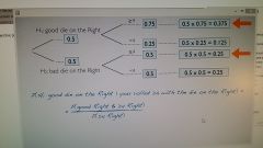
Week 03 What is the type 2 error rate? |
P(Type II error | HsubA is true) = beta. In other words, what is the probability that one will make a type two error, reject the alternative hypothesis when it's true.
This is also referred to as a 'false negative' rate. |
|
|
Week 03 Why do we prefer small values of alpha? |
To decrease the error rate (Type1 Error), when the stakes are high. |
|
|
What is the type 1 error rate? |
P(Type I error | HsubKnot is true) = alpha. In other words, what is the probability that one will make a type one error? |
|
|
What is beta in terms of the status quo? |
the probability of rejecting HsubA when you shouldn't have or the probability of failing to reject HsubKnot (status quo) when you should have. |
|
|
How does one choose alpha? |
If a Type I error is dangerous or especially costly, choose a small significane level (e.g. .01 ). if a type 2 error is relatively more dangerous or much more costly, choose a higher significance level (e.g. .10) |
|
|
What is alpha? |
The probability of rejecting HsubKnot (significance level).
Keep in mind that low alpha equals high significance, and high alpha equals low significance.
Keep it tight. Turn alpha on and off appropriately. |
|
|
Week 03
What is beta in terms of the status quo? |
The probability of rejecting HsubA when you shouldn't have or the probability of failing to reject HsubKnot (status quo) when you should have. |
|
|
Week 03
What is the Power of a Test? |
The probability of CORRECTLY REJECTING HsubKnot and it is represented by 1-beta (read as 1 take away the beta, follower) |
|
|
Week 03
What is the effect size? |
The difference between the point estimate and the null size. If the average is very close to the null value it will be difficult to detect a difference (and reject HsubKnot). If there is a bigger different value from the null value, it will be easier to detect a difference. |
|
|
Week 03 What is an observation? |
Together all observations and the corresponding variables make up a sample or in the case of the population, all observations consist of the entire population. |
|
|
Week 03 Kurtosis |
n probability theory and statistics, kurtosis (from Greek: κυρτός, kyrtos or kurtos, meaning "curved, arching") is any measure of the "peakedness" of the probability distribution of a real-valued random variable.[1] In a similar way to the concept of skewness, kurtosis is a descriptor of the shape of a probability distribution and, just as for skewness, there are different ways of quantifying it for a theoretical distribution and corresponding ways of estimating it from a sample from a population. There are various interpretations of kurtosis, and of how particular measures should be interpreted; these are primarily peakedness (width of peak), tail weight, and lack of shoulders (distribution primarily peak and tails, not in between). |
|
|
Week 03 Conjecture |
A conjecture is a proposition that is unproven. Karl Popper pioneered the use of the term "conjecture" in scientific philosophy.[1] Conjecture is related to hypothesis, which in science refers to a testable conjecture. In mathematics, a conjecture is an unproven proposition that appears correct |
|
|
Week 03 Conjecture |
A conjecture is a PROPOSITION that is UNPROVEN. Karl Popper pioneered the use of the term "conjecture" in scientific philosophy.[1]
Conjecture is related to hypothesis, which in science refers to a testable conjecture.
In mathematics, a conjecture is an UNPROVEN PROPOSITION that APPEARS correct. |
|
|
Conjecture |
A conjecture is a proposition that is unproven. Karl Popper pioneered the use of the term "conjecture" in scientific philosophy.[1] |
|
|
Kurtosis |
In probability theory and statistics, kurtosis (from Greek: κυρτός, kyrtos or kurtos, meaning "curved, arching") is any measure of the "peakedness" of the probability distribution of a real-valued random variable.[1]
There are various interpretations of kurtosis, and of how particular measures should be interpreted; these are primarily peakedness (width of peak), tail weight, and lack of shoulders (distribution primarily peak and tails, not in between). |
|
|
Generally, how are hypothesis test conducted? |
1. SIMULATION as with the example at the end of unit one where 48 cards were used to show promotions rates between men and women where a face card was not promoted and a non-face card was promoted. |
|
|
Week 03 We can use the ______________ to construct the sampling distribution when the null hypothesis is assumed to be true. |
Central Limit Theorem |
|
|
Alternative hypothesis is often represented by a ________ of possible values. They are ______________ |
range, <,> or not equal to. |
|
|
How does one read x bar ~ N( mu = 3, SE = .246 )? |
x bar nearly normally distributed with mu = 3 and the SE = .246. |
|
|
Week 03 Discrete Random Variable |
A discrete random variable is one which may take on only a COUNTABLE number of distinct values such as 0, 1, 2, 3, 4, ... Discrete random variables are USUALLY (but not necessarily) counts. If a random variable can take only a finite number of distinct values, then it must be discrete. Examples of discrete random variables include the number of children in a family, the Friday night attendance at a cinema, the number of patients in a doctor's surgery, the number of defective light bulbs in a box of ten. |
|
|
What does a negative vs positive z-score mean? |
It means the point estimate (sample mean) is left or right, respectively, of the population mean. |
|
|
What does correlation refer to? |
Refers to any of a broad class of statistical relationships involving which may or may not involve dependence. |
|
|
Discrete Random Variable |
A discrete random variable is one which may take on only a countable number of distinct values such as 0, 1, 2, 3, 4, ... Discrete random variables are usually (but not necessarily) counts. If a random variable can take only a finite number of distinct values, then it must be discrete. |
|
|
Continous Random Variable |
A continuous random variable is one which takes an INFINITE number of possible values. Continuous random variables are usually measurements. Examples include height, weight, the amount of sugar in an orange, the time required to run a mile. |
|
|
Descriptive vs Inferential (Inductive) Statistics |
Descriptive statistics are distinguished from inferential statistics (or inductive statistics), in that descriptive statistics aim to SUMMARIZE a sample, rather than use the data to learn about the population that the sample of data is thought to represent. |
|
|
Quantitative vs. Visual Summaries |
Descriptive statistics that provides summaries fall into two categories: |
|
|
Week 03 Observational Study |
Collect data in a way that does not directly interfere with how the data arise ("observe") |
|
|
Quantitative vs. Visual Summaries |
Descriptive statistics that provides summaries fall into two categories: or |
|
|
Week 03 Does the Central Limit Theorem apply to the median or mean? |
Mean. It cannot be used with the median. |
|
|
Week 04 What is bootstrapping? |
It is a concept that is used in testing a hypothesis when working with the median as opposed to the mean.
It comes from the widely known meaning of pulling oneself up by the boot straps to accomplish, basically, an impossible task. |
|
|
Random Assignment |
Taking a random sample of a population and then randomly assigning to a group |
|
|
Week 04 How does one bootstrap? |
Sample the sample. |
|
|
Random Assignment |
Taking a random sample of a population and then randomly assigning to a group |
|
|
Week 04 What does having a SPECIAL CORRESPONDENCE mean? |
They are not independent. They are paired (dependent). |
|
|
Week 04 Should the order of subtraction when using paired data be consistent? |
Yes. |
|
|
Week 04 Parameter of interest |
Average difference between paired data of the observations in a population. It's represented by
Mu(diff) |
|
|
Week 04 Point estimate for paired data |
Average difference between paired data taken from a sample of a population. It's represented by
x-bar (diff) |
|
|
Should the order of subtraction, when using paired data, be consistent? |
Yes. |
|
|
Alternative Hypothesis for paired means |
There's something going on. In the example with high school students looking at reading and writing scores, therefore,
HsubA: Mu(diff) does not equal 0 (there is a difference) |
|
|
Week 04 Do we use the Central Limit Theorem with paired data. |
Yes, after boiling down the data to one variable as was the case with the example of reading and writing scores with high school students.
Important to note that we started with two dependent variables and reduced them down to independent variables which is a condition of the CLT. |
|
|
Week 04 What are applications of paired data? |
|
|
|
Statistically, what does the alternative hypothesis for paired means represent? |
There's something going on. In the example with high school students looking at reading and writing scores, therefore,
HsubA: Mu(diff) does not equal 0 (there is a difference) |
|
|
Do we use the Central Limit Theorem with paired data? |
Yes, after boiling down the data to one variable as was the case with the example of reading and writing scores with high school students. |
|
|
What are applications of paired data? |
1. Pre-post studies such as weight loss over a period |
|
|
Week 04 What does it mean if one has a 95% confidence interval for (Mu(read) - Mu(write)) = (-1.78,0.69)? |
We are 95% confident that the difference between the average reading and writing scores is between -1.78 and 0.69 points. |
|
|
Week 04 Ordinal Variable |
An ordinal variable is similar to a categorical variable. The difference between the two is that there is a clear ordering of the variables. For example, suppose you have a variable, economic status, with three categories (low, medium and high). In addition to being able to classify people into these three categories, you can order the categories as low, medium and high. Now consider a variable like educational experience (with values such as elementary school graduate, high school graduate, some college and college graduate). These also can be ordered as elementary school, high school, some college, and college graduate. Even though we can order these from lowest to highest, the spacing between the values may not be the same across the levels of the variables. Say we assign scores 1, 2, 3 and 4 to these four levels of educational experience and we compare the difference in education between categories one and two with the difference in educational experience between categories two and three, or the difference between categories three and four. The difference between categories one and two (elementary and high school) is probably much bigger than the difference between categories two and three (high school and some college). In this example, we can order the people in level of educational experience but the size of the difference between categories is inconsistent (because the spacing between categories one and two is bigger than categories two and three). If these categories were equally spaced, then the variable would be an interval variable. |
|
|
Week 04 Interval Variable |
An interval variable is similar to an ordinal variable, except that the intervals between the values of the interval variable are equally spaced. For example, suppose you have a variable such as annual income that is measured in dollars, and we have three people who make $10,000, $15,000 and $20,000. The second person makes $5,000 more than the first person and $5,000 less than the third person, and the size of these intervals is the same. If there were two other people who make $90,000 and $95,000, the size of that interval between these two people is also the same ($5,000). |
|
|
Week 04 Parameter of interest for two independent variables for instance college degree and no college degree. |
Mu(coll) - Mu(no coll) |
|
|
Week 04 Point estimate for two independent variables for instance college degree and no college degree. |
point estimate +- margin of error
(x-bar(1) - x-bar(2) +- z*SE(x-bar(1) - x-bar(2))
|
|
|
Week 04 Standard error of difference between two independent means |
SE(x-bar(1) - x-bar(2)) = sqrt(std(1)^2/n(1)+std(2)^2/n(2))
Notice that while we are subtracting the means we are adding the variances because bringing them together there should be more variance. |
|
|
Week 04 How does one combine two parameters of interest such as instance two independent variables for comparison like college degree and no college degree. |
Mu(coll) - Mu(no coll) |
|
|
Week 04 What is the z*, critical value, for a 95% confidence interval?
|
1.96 |
|
|
Week 04 How would one interpret the confidence interval (0.66, 4.14) when comparing the difference in hours worked between independent variables of college-degree (no of hours worked/wk) to non college-degree (no of hours worked/wk) |
On average, college graduates work .66 to 4.14 more hours per week if one were to take a sample from the two independent groups. |
|
|
Week 04 What is a measure of central tendency? |
It is a single value that attempts to describe a set of data by identifying the central position within that set of data.
As such, measures of central tendency are sometimes called measures of central position, also classed as summary statistics.
Definition taken from:
https://statistics.laerd.com/statistical-guides/measures-central-tendency-mean-mode-median.php |
|
|
Week 04 When would one not want to use the mean? |
The mean has one main disadvantage: it is particularly susceptible to the influence of outliers. These are values that are unusual compared to the rest of the data set by being especially small or large in numerical value. For example, consider the wages of staff at a factory below:
Staff of 10 people with the following salaries: Salary 15k 18k 16k 14k 15k 15k 12k 17k 90k 95k
The mean salary for these ten staff is $30.7k. However, inspecting the raw data suggests that this mean value might not be the best way to accurately reflect the typical salary of a worker, as most workers have salaries in the $12k to 18k range. The mean is being skewed by the two large salaries. Therefore, in this situation, we would like to have a better measure of central tendency. As we will find out later, taking the median would be a better measure of central tendency in this situation. Another time when we usually prefer the median over the mean (or mode) is when our data is skewed (i.e., the frequency distribution for our data is skewed). If we consider the normal distribution - as this is the most frequently assessed in statistics - when the data is perfectly normal, the mean, median and mode are identical. Moreover, they all represent the most typical value in the data set. However, as the data becomes skewed the mean loses its ability to provide the best central location for the data because the skewed data is dragging it away from the typical value. However, the median best retains this position and is not as strongly influenced by the skewed values. This is explained in more detail in the skewed distribution section later in this guide. |
|
|
Week 04 What is bootstrapping? |
An alternative approach to sampling distribution by sampling the sample, hence, the term bootstrap. |
|
|
Week 04 How does the bootscrapping scheme work? |
1. Take a bootstrap sample - a random sample taken WITH REPLACEMENT from the original sample of the same size as the original sample
2. calculate the bootstrap statistic - a statistic such as mean, median, proportion, etc. computed on the bootstrap samples
3. repeat steps (1) and (2) many times to create a bootstrap distribution - distribution of bootstrap statistics |
|
|
Week 04 When would one not want to use the mean? |
The mean has one main disadvantage: it is particularly susceptible to the influence of OUTLIERS. These are values that are unusual compared to the rest of the data set by being especially small or large in numerical value. For example, consider the wages of staff at a factory below:
Staff of 10 people with the following salaries: Salary 15k 18k 16k 14k 15k 15k 12k 17k 90k 95k
The mean salary for these ten staff is $30.7k. However, inspecting the raw data suggests that this mean value might not be the best way to accurately reflect the typical salary of a worker, as most workers have salaries in the $12k to 18k range. The mean is being skewed by the two large salaries. Therefore, in this situation, we would like to have a better measure of central tendency. As we will find out later, taking the median would be a better measure of central tendency in this situation. Another time when we usually prefer the median over the mean (or mode) is when our DATA'S SKEWED (i.e., the frequency distribution for our data is skewed). If we consider the normal distribution - as this is the most frequently assessed in statistics - when the data is perfectly normal, the mean, median and mode are identical. Moreover, they all represent the most typical value in the data set. However, as the data becomes skewed the mean loses its ability to provide the best central location for the data because the skewed data is dragging it away from the typical value. However, the median best retains this position and is not as strongly influenced by the skewed values. This is explained in more detail in the skewed distribution section later in this guide. |
|
|
Week 04 What are the two methods for determining the confidence interval for bootstrapping? |
1. Percentile Method 2. Standard method using computation as opposed to the CLT. |
|
|
Week 04 Describe the percentile method of bootstrapping? |
Assume a 90% bootstrap confidence interval and 100 samples from the original sample then multiply the confidence interval by the # of samples
100 x .90 Subtract the result from the original sample 100-90 = 10 Divide the result by 2 to represent both sides of distribution 10/2 = 5 Then find the 5th percentile and 95th percentile. The corresponding numerical values represent the upper and lower bounds of the confidence intervals.
For instance, if working with median prices of apartments from the example in Unit 04 Part 02 Bootscrapping, then those would be
($740,$1050)
To characterize the data, we'd be 90% confident that the median value of an apartment in Durham would be between these values. |
|
|
Week 04 What does with replacement do with bootstrapping? |
It simulates taking many more samples than the one the researcher is working with. It assumes that is another sample was taken, the data would show that there would be another similar apartment to the one that is being replaced (put back) in the original sample, hence, the simulation of taking other samples. |
|
|
Week 04 What is a limitation of the bootstrap method compared to the CLT? ( 1 of 3 limitations of bootstrapping) |
The conditions are not as rigid. |
|
|
Week 04 When would the bootstrap method become unreliable? (1 of 3 limitations of bootstrapping) |
if the distribution is extremely skewed or sparse. |
|
|
Describe the standard error method for the bootscrap method using a 90% confidence interval? |
It is important that the SE is taken from the result of the bootscrap distribution, resulting from the plot of all the samples used to build the distribution. |
|
|
When would the bootstrap method becomes unreliable? (1 of 3 limitations of bootstrapping) |
If the distribution is extremely skewed or sparse. |
|
|
Week 04 t-distribution |
focuses on the mean and is used with small sample sizes. |
|
|
Describe the standard error method for the bootstrap method using a 90% confidence interval? |
It is important that the SE is taken from the result of the bootstrap distribution, resulting from the plot of all the samples used to build the distribution. |
|
|
Week 04 When would one use the t distribution? |
|
|
|
When would the bootstrap method become unreliable? (1 of 3 limitations of bootstrapping) |
If the distribution is extremely skewed or sparse. |
|
|
Week 04 What is unimodal? |
having or involving one mode. of a statistical distribution, having one maximum |
|
|
Week 04 Why would an standard error estimate be less reliable for a t distribution? |
because n is small. with a small sample, it naturally follows that the standard error would be less reliable.
Think back to the equation for standard error where as n becomes larger the standard error becomes smaller (more reliable, precise and accurate assuming the data is good data) |
|
|
Week 04 How many parameters does the normal distribution have? |
Two, the mean and the standard deviation |
|
|
Week 04 What is the relationship of the shape of a t-distribution and the degrees of freedom (df)? |
They are inversely proportional, comparing the tail of the distribution to the degrees of freedom
df = 1/tail thickness
Another way to look at a high degree of freedom is the tails get smaller, squeezing out the possibility of an outlier occuring. |
|
|
Week 04 What is unimodal? |
having or involving one mode of a statistical distribution, having one maximum |
|
|
Week 04 How is the t-statistic calculated? |
The same as the z statistic
T = obs - null/SE where obs is observed and null is the null hypotheis ( HsubKnot )
|
|
|
Week 04 How does one define the p-value for a t distribution |
It is the same definition as a normal distribution and the t - statistic could look at
|
|
|
Week 04 How does one calculate the p-value for a t statistic? |
Using R, applet or table. |
|
|
Week 04 Describe the relationship of the degrees of freedom a t-distribution to the sample size |
There are proportional; that is, as sample size goes up the degrees of freedom go up. |
|
|
Week 04 Interpret the following z statistic the to t statistic with different degrees of freedom
A. P(|Z| > 2) 0.0455 ------> reject? B. P(|t(df)=50| > 2) 0.0509 ------> fail to reject? C. P(|t(df)=10| > 2) 0.0734 ------> fail to reject? |
Even though all these examples have the same test statistic value, notice that the z-statistic of A is more rigid whereas with the t statistic as the degrees of freedom become higher, the probability of rejecting the null becomes higher as well.
The probability that the test statistic falls outside of 2 get higher going from A to C. |
|

Week 04 What is the real name of the t distribution and where did it originate? |
The real name is Student's t. It comes from a pseudonym from William (Willy) Gosset (1876-1937) who worked for Guiness brewing company as the "Head Experimental Brewer" to keep Guisness' brew secret.
He worked on methods that used small samples because sometimes he would only have small batches of a new barley. |
|
|
Describe the relationship of the degrees of freedom a t-distribution to the sample size. |
There are proportional; that is, as sample size goes up the degrees of freedom go up. |
|
|
Week 04 Blocking |
In the statistical theory of the design of experiments, blocking is the arranging of experimental units in groups (blocks) that are similar to one another. For example, an experiment is designed to test a new drug on patient |
|
|
What is the real name of the t distribution and where did it originate? |
It comes from a pseudonym from William Gosset (1876-1937) who worked for Guiness brewing company as the "Head Experimental Brewer" called the |
|
|
Week 04 Formula to calculate the Degrees of freedom (df) for t statistic for inference on ONE sample mean |
df = n - 1.
We are losing one degree of freedom because we are dealing with the stddev from the sample which is fine because we've done that before. However, we are taking data from a small sample so we are hesitant because we are not absolutely certain the standard error represents the population. |
|
|
Week 04 How does one find the critical t score using the table? |
1. Determine df = n - 1 2. Find corresponding tail area for desired confidence level
|
|
|
Week 04 Interpret the following z statistic to the t statistic with different degrees of freedom
A. P(|Z| > 2) 0.0455 ------> reject? B. P(|t(df)=50| > 2) 0.0509 ------> fail to reject? C. P(|t(df)=10| > 2) 0.0734 ------> fail to reject? |
Even though all these examples have the same test statistic value, notice that the z-statistic of A is more rigid whereas with the t statistic as the degrees of freedom become higher, the probability of rejecting the null becomes higher as well.
The probability that the test statistic falls outside of 2 gets higher going from A to C. |
|
|
Week 04 Quantile |
Each of any set of values of a variate that divide a frequency distribution into equal groups, each containing the same fraction of the total population |
|
|
Describe the relationship of the degrees of freedom of a t-distribution to the sample size. |
They are proportional; that is, as sample size goes up the degrees of freedom go up. |
|
|
Week 04 Blocking |
In statistical theory of the design of experiments, blocking is the arranging of experimental units in groups (blocks) that are similar to one another. For example, an experiment is designed to test a new drug on patient |
|
|
Week 04 what is a Contradistinction? |
distinction made by contrasting the different qualities of two things. |
|
|
Week 04 What must one do when determining the probability |
Draw the distribution |
|
|
Week 04 What is a variate? |
|
|
|
What is a contradistinction? |
Distinction made by contrasting the different qualities of two things. |
|
|
What must one do when determining the probability? |
Draw the distribution. |
|
|
Week 04 What are the methods used in this course for hypothesis testing? 6 methods |
1. large sample ( CLT (nearly normal distribution) and z statistic 2. paired data ( use CLT ) 3. comparing independent means 4. median ( bootstrapping) 5. small sample ( t distribution ) 6. ANOVA (analysis of variance) |
|
|
Week 04 What does p stand for in pt or pnorm |
probability or percentile |
|
|
What is a construct? |
An idea or theory containing various conceptual elements, typically one considered to be subjective and not based on empirical evidence. |
|
|
Week 04 How does one construct the confidence interval for comparing means based on small samples |
point estimate +- margin of error
( x-bar(1) - x-bar(2) +- t*(df)SE( x-bar(1) - x-bar(2)) |
|
|
How does one determine the p-value using R for a t distribution? |
Use pt function which requires two arguments: |
|
|
Evaluate whether or not the following data would conform to a nearly normal distribution based on the 68.7%, 96, 99.7% rule. |
This would not conform to a normal distribution ( This is important when determining which hypothesis test method to use based on conditions such as CLT ) |
|
|
How does one construct the confidence interval for comparing means based on small samples? |
point estimate +- margin of error |
|
|
How does one calculate the t statistic for comparing means based on small samples |
T(df) = ( obs-null ) / SE |
|
|
Week 04 What does ANOVA stand for? |
Analysis of Variance. It is used to compare 3+ means |
|
|
How do one calculate the DF ( degrees of freedom ) for the t statistic for inference on two different means? |
df = min (n(1) - 1, n(2) - 1) |
|
|
Week 04 Using ANOVA, how would one represent the null hypothesis? |
HsubKnot: The mean outcome is the same across all categories
mu(1) = mu(2) = . . . = mu(k)
where k is the number of groups and mu(i) is the mean of the outcome for observations in category i (categorical variable) |
|
|
What does ANOVA stand for? |
Analysis of Variance, it s used to compare 3+ means |
|
|
Week 04 Do a contradistiction between z/t test and ANOVA |
z/t test
Compare means from two groups: are so far apart that the observed difference cannot reasonably be attributed to sampling variability?
HsubKnot mu(1) = mu(2)
ANOVA
Compare means from more than two groups: are they so far apart that the observed differences cannot all reasonably be attributed to sample variability?
HsubKnot mu(1) = mu(2) = . . . = mu(k) |
|
|
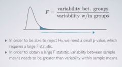
Week 04 How does one compute the F statistic for ANOVA |
Compute a test statistic ( a ratio )
F = variability between groups / variability w/in groups
F = MSG / MSE (Mean Square Group/Mean Square Error) |
|
|
Week 04 Do a contradistinction between z/t test to the F statistic |
They are all ratios
z/t test = ((x-bar(1) - x-bar(2)) - (mu(1) - mu(2)) / SE ( x-bar(1) - x-bar(2) )
F = variability between groups / variability w/in groups
|
|
|
Week 04 What is the relationship between large test statistics and p-values |
Large test statistics ALWAYS lead to small p-values. |
|
|
Week 04 If the p-value is small enough what can be concluded when comparing two means |
HsubKnot can be rejected and one can conclude that the data provide evidence of a difference in the population means when comparing two means. |
|
|
Week 04 What is a requirement for a large F statstic? |
Variability BETWEEN sample means needs to be greater than the variability WITHIN sample means. |
|
|
What is the relationship between large test statistics and p-values? |
Large test statistics ALWAYS lead to small p-values. |
|
|
Week 04 What are the three statistics used in this course? |
|
|
|
Week 04 What is variability partitioning? |
In the example of social class (explanatory variable) and vocabulary score ( response variable ), variability partitioning looks at the explanatory variable and determines what part of the score can be attributed to class ( BETWEEN GROUP VARIABILITY ) and what part of the score can be attributed to other factors ( WITHIN GROUP VARIABILITY study habits, etc )
|
|
|
Week 04 What is the sum of squares total, what is its abbreviation and how is it calculated? |
It measures the total variability in the response variable (social class for instance) and its abbreviation is SST, also called Total in ANOVA table
It's calculated very similarly to variance ( save it's not scaled by the sample size )
SST = Sum(i=1,n) (y(i) - y-bar)^2
where y(i) is the value of the response variable for each observation and y-bar is the grand mean of the response variable
Example follows:
1 6 2 9 3 6 . . . 795 9
n mean sd overall 795 6.14 1.98
SST = (6-6.14)^2 + (9-6.14)^2 + (6-6.14)^2 + . . . + (9-6.14)^2
|
|
|
Week 04 Does the SST mean anything by itself? |
No. |
|
|
Week 04 What is the sum of squares groups, its meaning and its abbreviation? |
|
|
|
Week 04 How does one calculate the Sum of squares Group (SSG) |
SSG = sum(j=1,k) n(j)*(y-bar(j)-y-bar)^2
where n(j) is the number of observations in group j where y-bar(j) is the mean of the response variable for group j and where y-bar is the grand mean of the response variable
Example follows:
n mean sd lower class 41 5.07 2.24 working class 407 5.75 1.87 middle class 331 6.76 1.89 upper class 16 6.19 2.34 overalll 795 6.14 1.98
SSG = 41(5.07-6.14)^2 + (407*(5.75-6.15)^2) + (331*(6.76-6.14)^2 + (16*(6.19-6.14)^2) = 236.56
By itself this is again not a meaning number. |
|
|
Week 04 Describe the ANOVA table |
There are 2 rows and 5 cols
2 rows, Group and Error 5 rows
The rows add up the totals shown in the last row.
|
|
|
Week 04 In the ANOVA table what is another name for the Error row? Are we interested in this and what does it represent. |
Residuals. We are not interested in this and it is the WITHIN GROUP variability that we are not interested in because of the other factors |
|
|
Week 04 What is variability partitioning? |
In the example of social class (explanatory variable) and vocabulary score ( response variable ), variability partitioning looks at the explanatory variable and determines what part of the score can be attributed to class ( BETWEEN GROUP VARIABILITY ) and what part of the score can be attributed to other factors ( WITHIN GROUP VARIABILITY study habits, etc ). As the name implies, it parcels variability to the between group or across group components.
|
|
|
How does one calculate the Sum of Squares Group (SSG)? |
SSG = sum(j=1,k) n(j)*(y-bar(j)-y-bar)^2 |
|
|
Week 04 What is the mean square error associated with ANOVA and how are they calculated? |
Average variability between and within groups, calculated as the total variability (sum of squares) scaled by the associated degrees of freedom.
|
|
|
Week 04 What is the sum of squares groups, its meaning and its abbreviation? |
|
|
|
Week 04 How does one calculate the Sum of Squares Group (SSG) |
SSG = sum(j=1,k) n(j)*(y-bar(j)-y-bar)^2
where n(j) is the number of observations in group j where y-bar(j) is the mean of the response variable for group j and where y-bar is the grand mean of the response variable
Example follows:
n mean sd lower class 41 5.07 2.24 working class 407 5.75 1.87 middle class 331 6.76 1.89 upper class 16 6.19 2.34 overall 795 6.14 1.98
SSG = 41(5.07-6.14)^2 + (407*(5.75-6.15)^2) + (331*(6.76-6.14)^2 + (16*(6.19-6.14)^2) = 236.56
By itself this is again not a meaning number. |
|
|
Week 04 Describe the ANOVA table |
There are 2 rows and 5 cols
2 rows, Group and Error 5 rows
The rows add up to the totals shown in the last row.
|
|
|
Week 04 What does the F distribution look like? |
It is right skewed. |
|
|
Week 04 Are there any two-tailed hypothesis test with the F distribution? |
No. |
|
|
How would one interpret F(3,791) for an F distribution? |
F distribution with a group degrees of freedom of 3 and 791 degrees of freedom for the error. |
|
|
Week 04 What is the mean square error and mean square group associated with ANOVA and how are they calculated? |
Average variability between and within groups, calculated as the total variability (sum of squares) scaled by the associated degrees of freedom.
|
|
|
Week 04 What is the max degrees of freedom (E) in the online app? Is this a hindrance? |
120. no. You'll have to reason through the visual that is presented. |
|
|
Week 04 What are the conditions for ANOVA? |
BETWEEN Groups - the groups must be independent of each other (non-paired) 2. Approximate Normality 3. Equal Variance - groups should have roughly equal variability. |
|
|
What are the 3 degrees of freedom associated with ANOVA? |
Total df(T) = n-1 where n is the number of observations in the sample |
|
|
Week 04 What are repeated measures ANOVA? |
This looks at the independence condition of ANOVA where instead of having no pairing, there's pairing.
Will not be covered in this course. |
|
|
Week 04 Describe the approximately Normal condition for ANOVA? |
One way to check is to look at a normal probability plot ( the line and adherence to it ) |
|
|
Week 04 Describe the constant variance condition for ANOVA |
|
|
|
Week 04 What is homoscedastic and to which hypothesis testing method would that apply? |
It means variability across groups should be consistent.
It would apply to the F distribution. |
|
|
Week 04 How can homoscedastic be checked? |
By looking at side by side box plots of each group being considered in a study.
Visualize a boxplot and how one could easily see the variability between groups, standard deviations, and sample sizes. |
|
|
Week 04 What is a way of reducing Type I error when doing multiple comparisons |
Use a modified siginificance level |
|
|
Week 04 What is multiple comparisons? |
Testing many pairs of groups. |
|
|
Week 04 What does the Bonferroni correction suggests? |
That a more stringent significance level is more appropriate for multiple comparison tests.
This makes sense to avoid magnifying the probability of a Type I error. |
|
|
Week 04 Describe the approximately Normal condition for ANOVA? |
One way to check is to look at a normal probability plot ( the line and adherence to it ) |
|
|
Week 04 Describe the constant variance condition for ANOVA. |
|
|
|
Week 04 What is the degrees of freedom for multiple pairwise comparisons using ANOVA? |
Regardless of the comparisons, the degrees of freedom from the ANOVA output is the same for all comparisons
df = df(E) |
|
|
Week 04 What does a test statistic represent? |
The number of stddev from the mean. This is why a high test statistic makes the chances of an occurence happening that far from the mean very slim.
|
|
|
Week 04 What is the summary function and what is the notation? |
Used to summarize a dataset, including mean, 3rd quartile, max, NA's, min, and 1st quartile of each variable in a dataset |
|
|
Week 04 What is another name for a dataset? |
dataframe |
|
|
Week 04 What is the boxplot function and the syntax? |
It graphically represents the data in a boxplot format. The syntax is:
boxplot(nc$habit, nc$weight) where habit and weight are categorical and numerical variables, respectively, in the nc dataset |
|
|
Week 04 How does one identify a variable in R? |
It must be prefaced by the dataset owing the variable and then its name separated with a dollar sign as follows:
nc$habit
This represents the variable habit in the dataframe nc. |
|
|
Week 04 What is the by function in R and describe the syntax? |
The representation is as follows:
|
|
|
Week 04 What is the inference function describe it's arguments and syntax? |
The inference function for evaluating whether there is a difference between the mean of a numerical variable common to a categorical variable with obvious different characteristics such as a smoker and non-smoker.
In this case, the birth weights of babies born to smoker and non-smoker mothers. Let’s pause for a moment to go through the arguments of this custom function:
inference(y = nc$weight, x = nc$habit, est = "mean", type = "ht", null = 0, alternative = "twosided", method = "simulation") |
|
|
Week 04 What is theoretical vs. simulation? |
Theoretical involves sample from the population with replacement.
Simulation involves a sample from the sample with replacement. |
|
|
Week 04 What is the summary function and what is the notation? |
Used to summarize a dataset, including mean, 3rd quartile, max, NA's, min, and 1st quartile of each variable in a dataset
summary(dataset) |
|
|
Week 04 What is the syntax for loading a dataset into R? |
load(url("link_to_dataset")). Important: Don't forget the quotes. |
|
|
Week 04 What are boxplots good for? |
Plotting a numerical, y axis, vs. a categorical variable, x axis. |
|
|
Week 04 What are histograms good for? |
Plotting the frequency of a discrete numerical variable such as a test score where only whole numbers are allowed.
e.g. The number of correct answers on a test vs the number of times (frequency) that it occurred. |
|
|
Week 04 What is the by function in R and describe the syntax? |
The representation is as follows:
|
|
|
Week 04 Of the hypothesis testing that we used in this course, which method is appropriate for testing for a difference between the average vocabulary test scores among the various social classes? |
ANOVA, consider the number of levels of the class variable. |
|
|
Week 04 What is theoretical vs. simulation? |
Theoretical involves SAMPLE FROM THE POPULATION with replacement.
Simulation involves a SAMPLE FROM THE SAMPLE with replacement. |
|
|
Week 04 Conditions for using the t - interval |
Conditions to use the t-interval are:
|
|
|
Week 05 What are characteristics of a count variable? |
In statistics, count data is a statistical data type, a type of data in which the observations can take only the non-negative integer values {0, 1, 2, 3, ...}, and where these integers arise from counting rather than ranking. The statistical treatment of count data is distinct from that of binary data, in which the observations can take only two values, usually represented by 0 and 1, and from ordinal data, which may also consist of integers but where the individual values fall on an arbitrary scale and only the relative ranking is important. |
|
|
Week 05 Describe what two levels would be in terms of a categorical variable?
Can a categorical variable take on more than two levels? |
Two levels of a categorical variable would be the different categories (distinctions) within the variable.
For instance, it could be success-failure where success doesn't necessarily represent something some positive such as someone dying.
Categorical variables can take on more than two levels like economic status such as low, medium or high. |
|
|
Week 05 Do categorical variables have means?
What represents the mean (sample statistic) with categorical variables? |
No. The sample proportion is used in lieu of a mean with categorical variables since means cannot sensibly be calculated with a categorical variable. |
|
|
Week 05 Is the sample proportion a sample statistic? How is it represented |
Yes. It is represented as a proportion. For example, in a sample, with n observations, the proportion (p) is the percentage of the sample represented by the categorical characteristic, like being a smoker, of the entire sample as follows
p = # of smokers/sample size |
|
|
Week 05 Does the definition of sample distribution and sampling distribution change from categorical variables?
What is a characteristic of a sampling distribution? |
No. The sample statistic, for instance, the sample proportion, is characteristically a sampling distribution.
For example, one could in theory determine all the people in the world who smoke in which you'd be taken a sample distribution
OR
You could do a sample of three countries like Afghanistan, the US and Zimbabwe in which case this would be a sampling distribution.
|
|
|
Week 05 Which theorem applies to sample proportions? |
The Central Limit Theorem. |
|
|
Week 05 How does the central limit theorem describe the distribution for a sample proportion?
What 3 characteristics of the sample are determined? |
The CLT states that a distribution of sample proportions is nearly normal, centered at the population proportion, and with a standard error inversely proportional to the sample size.
P(hat) ~ N(mean = p, SE (standard error = sqrt(p(1-p)/n))
|
|
|
Week 05 What are the conditions for the CLT as it applies to a categorical variable? |
|
|
|
Week 05 Describe what two levels would be in terms of a categorical variable?
Can a categorical variable take on more than two levels? |
Two levels of a categorical variable would be the different categories (distinctions) within the variable.
For instance, it could be success-failure where success doesn't necessarily represent something positive such as someone dying.
Categorical variables can take on more than two levels like economic status such as low, medium or high. |
|
|
Week 05 When would one use the binomial probability distribution and what is the function in R? |
The binomial probability distribution is useful when a total of n independent trials are conducted and we want to find out the probability of r successes, where each success has probability p of occurring. There are several things stated and implied in this brief description. The definition boils down to these four conditions:
In R, the function takes 3 arguments
1. The range of the alternative hypothesis that defines the probability of finding the observed or more extreme outcome. The example in the videos described that 90% of all plants species are classified as angiosperms (flowering plants) 2. The sample size, in this case, 200. 3. The null hypothesis (probability), 90%
> sum(dbinom(*190:200, 200, 0.90) [1] .00807125
This is the same answer given if one were to use the z score, the quantile where the observed or more extreme outcome would occur. So, the value give by dbinom is the area under the curve beyond 95%. |
|
|
Week 05 What if the success-failure condition of the CLT is not met? |
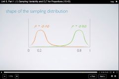
Notice from the diagram that the closer one moves toward 1 the sample becomes more left skewed and as one's sample becomes closer to 0 the sample between comes more right skewed.
|
|
|
Week 05 How does one load excel data into R? |
Through the menu bar. |
|
|
Week 05 Can sample proportions be greater than 1 or less than 0? |
No. This makes sense since the sample proportion represents a probability, and we know that a probability must be between zero and 1. |
|
|
Week 05 How does one calculate the confidence interval for a proportion? |
x(bar) +- margin error x(bar) +- z* SE x(bar) =- z* sqrt(p(1-p)/670)
|
|
|
Week 05 What are the 2 possibilities of data we would use to calculate the required sample size for a desired ME (margin of error)? |
|
|
|
Week 05 parameter of interest as compared to the point estimate for difference in proportions |
Average difference between data which may or may not have a dependence, of the observations in a population. It's represented by
Mu(diff)
In the video, Unit 5 Part 2 Section 1, the questions posed was how do Coursera students and the American public at large compare with respect to their views on laws banning possession of handguns
The parameter of interest in this case is the difference between the proportions of ALL Coursera students and ALL Americans who believe there should be a ban on possession of handguns, represented by
p(coursera) - p(us)
The point estimate is the difference between the proportions of SAMPLED Coursera students and SAMPLED Americans who believe there should be a ban on possession of handguns.
p(coursera)- p(us) |
|
|
Week 05 What are the steps for a Hypothesis Test for a single categorical variable? |
|
|
|
Week 05 When does one use p and when does one use p(hat)? |
____________________________| confidence interval | hypothesis test ____________________________|_____________________|__________________ success-failure condition__| ______np(hat)>=10__|_____np>=10 ____________________________|____n(1-p(hat)>=10__|___n(1-p)>=10__| ____________________________|_____________________|__________________ _________standard error____| SE(hat)____________|_____SE ____________________________|_____________________|____________________ |
|
|
Week 05 What is the formula for calculating sample proportions point estimate between two independent variables |
point estimate +- margin of error
p1(hat) - p2(hat) +- z* SE(p1(hat)-p2(hat))
SE = sqrt((p1(hat)(1-p1(hat))/n1) + (p2(hat)(1-p2(hat))/n1)) |
|
|
Week 05 What is the pooled proportion to determine the null hypothesis for the hypothesis test? |
In contrast to what has been learned up to this point, it is a way of using the sample statistic to help in determining the population parameter or interest when working with the sample proportion.
So, H(null) is not given so using the sample statistic one is able to come up with a "best guess" |
|
|
Week 05 What is the formula for the pooled proportion: |
p(hat)pool = total successes/total n
____________= (number of successes(1) + # of successes(2)) / n(1) + n(2) |
|
|
Week 01 What does the command "head" do in R? |
It shows the first few rows of observations. |
|
|
Week 01 What does the # sign do in R? |
It "comments" an item. |
|
|
Week 05 How could one calculate a proportion using R? |
proportion = nrow(subset(us12,response == 'atheist'))/nrow(us12)
Note proportion becomes an object that previously was undefined.
Results
|
|
|
Week 05 How does one create a sequence of numbers separated by 0.01 with a range of 0 to 1? |
p = seq(0, 1, 0.01) |
|
|
Week 05 How does one plot two vectors against each other to reveal their relationship: |
# The first step is to make a vector p that is a sequence from 0 to 1 with each number separated by 0.01: # We then create a vector of the margin of error (me) associated with each of these values of p using the familiar approximate formula (ME = 2 X SE):
# Finally, plot the two vectors against each other to reveal their relationship:
|
|
|
Week 05 What is the pooled proportion to determine the null hypothesis for the hypothesis test? |
In contrast to what has been learned up to this point, it is a way of using the sample statistic to help in determining the population parameter of interest when working with the sample proportion.
So, H(null) is not given so using the sample statistic one is able to come up with a "best guess" |
|
|
Week 03 Experimental Study |
There is random assignment. The researcher "controls" how the data of the study is collected. |
|
|
Week 06 What is correlation between numerical variables? |
linear, negative, moderately |
|
|
Week 06 What is a linear correlation? |
It is either linear or non-linear.
|
|
|
Week 06 What is a negative or positive correlation? |
Negative means one numerical variable is increasing while the other is decreasing. Positive means both are increasing in the same direction. |
|
|
Week 06 What is moderately strong vs strong for correlation? |
If there's not much scatter then the relationship is strong. Otherwise, it is weak. |
|
|
Week 06 What does residuals mean in correlation? |
It is the model fit. It is the difference between the observed vs. the predicted (expected) |
|
|
Week 06 What is the representation for predicted and observed in correlation? |
The observed is p and the predicted is p-hat. |
|
|
Week 06 Can one just add up the residuals to get to the |
No. |
|
|
Week 06 What are the methods for the residuals in regression? |
|
|
|
Week 06 What is the equation for the least squares line? |
Y-hat = B(knot) + B(1)X
where y-hat is predicted response, B(knot) is the y - intercept, B(1) is the slope and x is the explanatory variable. |
|
|
Week 06 What is the notation for observed and point estimates? |
observed______point estimate B(zero)________b(zero) B(1) b(1) |
|
|
Week 06 What is the formula for the slope? |
rise over run
b1 = s(y)*R/S(x) |
|
|
Week 06 How would one interpret 62% living in poverty to high school education. |
For each % point increase in HS graduation rate, we would expect the % living in poverty to be lower on average by 62% points.
where 3.1%*.75/3.73% = 62% |
|
|
Week 06 With correlation, the regression line always goes through the ____________ of the data. |
center |
|
|
Week 06 What is the code for correlation in R? |
cor(mlb11$runs, mlb11$at_bats)
# print the correlation correlation |
|
|
Week 06 Use the following function to select the line that you think does the best job of going through the cloud of points.
plot_ss(x = mlb11$at_bats, y = mlb11$runs, x1, y1, x2, y2)
This function will first draw a scatterplot of the first two arguments x and y. Then it draws two points (x1, y1) and (x2, y2) that are shown as red circles. These points are used to draw the line that represents the regression estimate. The line you specified is shown in black and the residuals in blue. Note that there are 30 residuals, one for each of the 30 observations. Recall that the residuals are the difference between the observed values and the values predicted by the line: ei=yi−yi^
The most common way to do linear regression is to select the line that minimizes the sum of squared residuals. To visualize the squared residuals, you can rerun the plot_ss command and add the argument showSquares = TRUE.
plot_ss(x = mlb11$at_bats, y = mlb11$runs, x1, y1, x2, y2, showSquares = TRUE)
Note that the output from the plot_ss function provides you with the slope and intercept of your line as well as the sum of squares. |
plot_ss(x = mlb11$at_bats, y = mlb11$runs, x1, y1, x2, y2, showSquares = TRUE) # This is another one:
Call: lm(formula = y ~ x, data = pts) Coefficients: (Intercept) x 2550.0000 -0.3333 Sum of Squares: 302572.3> > # This is another one: > plot_ss(x = mlb11$at_bats, y = mlb11$runs, 5400, 550, 5700, 650, showSquares = TRUE) Call: lm(formula = y ~ x, data = pts) Coefficients: (Intercept) x -1250.0000 0.3333 Sum of Squares: 454843 |
|
|
Week 06 # Adapt the function to plot the best fitting line: |
plot_ss(x = mlb11$at_bats, y = mlb11$runs, leastSquares = TRUE, showSquares = TRUE) |
|
|
Week 06 What is the notation for observed and point estimates in a linear regain fit? |
observed______point estimate B(zero)________b(zero) B(1) b(1) |
|
|
Week 06 What is the formula for the slope? |
rise over run
b1 = s(y)*R/s(x) where s is respective the standard deviationfor each independent variable and R is the correlation between the two variables. |
|
|
Week 06 # Use the 'lm' function to make the linear model. |
Print the summary: |
|
|
Week 06
The function abline plots a line based on its slope and intercept. This line can be used to predict y at any value of x. When predictions are made for values of x that are beyond the range of the observed data, it is referred to as extrapolation and is not usually recommended. However, predictions made within the range of the data are more reliable. They're also used to compute the residuals
# The 'mlb11' data frame is already loaded into the workspace # Create a scatterplot: # The linear model: # Plot the least squares line: |
# The 'mlb11' data frame is already loaded into the workspace # Create a scatterplot: # The linear model: # Plot the least squares line: |
|
|
Week 06 To assess whether the linear model is reliable, you need to check for three things: |
To assess whether the linear model is reliable, you need to check for three things:
|
|
|
Week 06 You already checked if the relationship between runs and at-bats is linear using a scatterplot. You should also verify this condition with a plot of the residuals vs. at-bats. The lty=3 argument adds a horizontal dashed line at y = 0: plot(m1$residuals ~ mlb11$at_bats) abline(h = 0, lty = 3). |
You already checked if the relationship between runs and at-bats is linear using a scatterplot. You should also verify this condition with a plot of the residuals vs. at-bats. The lty=3 argument adds a horizontal dashed line at y = 0: plot(m1$residuals ~ mlb11$at_bats) abline(h = 0, lty = 3). |
|
|
Week 06
Point 2, nearly normal residuals: |
To check this condition, a normal probability plot of the residuals (the graph is shown). qqnorm(m1$residuals) qqline(m1$residuals) |
|
|
Week 06 Describe the impact of leverage |
The further away from from the mean of X (either in a |
|
|
Week 06 |
Based on a random sample of 170 married couples in Britain, a researcher finds that the relationship between the husbands’ and wives’ ages is described by the following equation: Most wives in Britain are 0.91 years younger than their husbands. On average, when a husband in Britain gets 1 year older, his wife only gets 0.91 years older. For each additional year increase of wife’s age, we would expect the husband’s age to be 0.91 years higher, on average. For each additional year increase of husband’s age, we would expect the wife’s age to be 0.91 years higher, on average. |
|
|
Week 07 What is multiple linear regression? |
Several explanatory variables and one response variable. |
|
|
Week 07 |
Multiple linear regression. |
|
|
Week 07 What is a predictor? |
An explanatory variable |
|
|
What does the following do?
# load data > library(DAAG) > data(allbacks)
#fit model >book_mlr = lm(weight ~ volume + cover, data = allbacks) |
look at the relationship between the volume of a book and it's volume |
|
|
Week 07 How many slopes does the following have?
weight - 97.06 + .72 volume - 185.05 cover:pb |
Two volume and cover:pb. This is the equivalent of having two x's or a function with more than one input. |
|
|
Week 06 Describe the impact of leverage |
The further away from from the mean of x (either in a |
|
|
Week 06 Based on a random sample of 170 married couples in Britain, a researcher finds that the relationship between the husbands’ and wives’ ages is described by the following equation: Which of the following is the best interpretation of the slope estimate?Most wives in Britain are 0.91 years younger than their husbands.On average, when a husband in Britain gets 1 year older, his wife gets a 1 year older keeping the expected difference in their age at 0.91 years. |
. Slope's rise over run. It keeps the spread in two variables the same. His wife gets a 1 year older keeping the expected difference in their age at 0.91 years.Slope's rise over run. It keeps the spread in two variables the same.The intercept displaces the line accordingly to represent the point estimate when the explanatory value is zero His wife gets a 1 year older keeping the expected difference in their age at 0.91 years.Slope's rise over run. It keeps the spread in two variables the same.The intercept displaces the line accordingly to represent the point estimate when the explanatory value is zero His wife gets a 1 year older keeping the expected difference in their age at 0.91 years.Slope's rise over run. It keeps the spread in two variables the same.The intercept displaces the line accordingly to represent the point estimate when the explanatory value is zero .Slope's rise over run. It keeps the spread in two variables the same.The intercept displaces the line accordingly to represent the point estimate when the explanatory value is zero The intercept displaces the line accordingly to represent the point estimate when the explanatory value is zero
|
|
|
Week 07 What is the not explained variability |
1 - adjusted. It is the complement to R squared. |
|
|
Week 07 How do we determine if the predictor is a useful one? |
adjusted R(squared) = 1 - (SSE/SST x n-1/n-k-1) where
k is the number of predictors. |
|
|
Week 07 What is the difference between r(squared) and adjusted r-squared? |
They are similiar in telling us about the percentage of variability but adjusted r(squared) has a penalty for the number of predictors in the model. |
|
|
Week 07 Properties of adjusted R-squared |
|
|
|
Week 07 What is collinearity? |
|
|
|
SE standard error in Regression Analysis |
In regression analysis, the term "standard error" is also used in the phrase standard error of the regression to mean the ordinary least squares estimate of the standard deviation of the underlying errors. |
|
|
Week 05 When dealing with categorical variables the point of interest is no longer a mean but a _______________. |
proportion |
|
|
Week 02 What is a probability tree? |
It is a way of graphically showing the probability of certain events happening, making it easier to organize the probabilities to be used in solving probability theory problems. |
|
|
Week 02 What is the third step usually in creating a probability tree? |
Calculate the joint probabilites by multiplying across the branches. See below which is a example that the professor gave in class of holding two dice one good (12-sided) and one bad (6-sided).
A game was played where the probability of rolling a number greater than 4 was determined. A probability tree was used to update the probability that the right hand was holding the good die and the left hand was holding the bad die.
This leads to a Bayesian inference. |
|
|
Week 02 What is the formula for Bayes theorem? |
multiply the probabilities / sum of the probabilities.
It says find the joint probability divided the marginal probability of B (all occurrences of B ) |
|
|
Week 02 What is a posterior probability? |
Bayes theorem constitutes a posterior probability.
It is generally defined as P (hypothesis|data).
It tells us the probability of a hypothesis we set forth, given the data we observed.
It is in contrast to the p-value which is P(data|hypothesis), that is, the probability of observed or more extreme data given the null hypothesis being true as in
P(data|hypothesis) |
|
|
Week 02 What are the advantages of a Bayesian approach? |
|
|
Week 7 Who is the Prince of Mathematics? Where did I learn this? |
The german, Karl Friedrich Gauss. He came up with the idea of least squared method used in linear regression.
I learned this from the audiobook Pricing the Future: Finance, Physics, and the 300-Year Journey to the Black-Scholes Equation |
|
|
What year did Gauss discover the method of least squares and what is the other well-known name of this method? |
1794, linear regression |
|
|
What is another name for linear regression and who discovered it? |
The method of least squares, Gauss. |
|
|
How did Gauss discover the method of least squares? |
When making an observation (e.g. GDP over time although this is no statement toward Gauss using this data) he noticed that the "best fitting" line can be fitted by minimizing the sum of squared differences of the observed values and the values on the line.
By squaring the differences, both the positive and negative values account for each other instead of zeroing each other out. |
|
|
Week 02 What is the formula for Bayes theorem? |
posterior probability / sum of the posterior probabilities that the evidence yield.
It says find the posterior probability divided the marginal probability of B (all occurrences of B ) where B is the evidence |
|
|
Week 01 Lab 1
|
information |
|
|
Week 01 Lab 1
What do the following functions do in R?
mean(cdc$weight) var(cdc$weight) median(cdc$weight)
table(cdc$smoke100) |
The functions do as the name implies. Remember R can evaluate expressions in the console so each of the function would return the corresponding value for a variable $variable in dataset cdc.
The key here is noting that the variable must be joined with the dataset. Remember inside OOP languages the scope of a variable is implied within a sub or procedure unless otherwise specified. One does not have to be this specific; however, this makes sense since these functions are being evaluated from the console.
The table function counts components of a categorical variable. In this case, how many people responded yes to having smoked a 100 cigarattes in their lifetime. |
|
|
Week 01 Lab 1
What does the following command do?
table(cdc&smoke100)/20000 |
It gives the relative frequence distribution in a data frame with 20000 observations as follows:
0 1
where 0 is no and 1 is yes, and there associated complimentary distributions to each other. |
|
|
Week 01 Lab 1
What does the following command do?
barplot(table(cdc$smoke100))
|
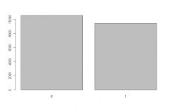
It creates a barplot of a table of categorical values as shown left. |
|
|
What would be the difference in the following commands
summary(cdc$gender) and table(cdc$gender) |
nothing the results of each follows:
> summary(cdc$gender) m f |
|
|
Week 01 Lab 1
What would the following yield?
table(cdc$genhlth)/20000
|
It creates a relative frequency distribution ( the total distribution sums to one) for the genhlth variable found in the cdc dataset
excellent very good good fair poor |
|
|
Week 01 Lab 1
What would the following do? Would it create a graph or initialize a variable?
gender_smokers = table(cdc$gender,cdc$smoke100) |
It creates a table where gender and smoke100 are associated. It initializes a variable holding table |
|
|
Week 01 Lab 1
Some define Statistics as the field that focuses on turning ______________ into knowledge. |
information |
|
|
OpenIntro Statistics Chapter 2 Probability (Special Topic), p 100
What is a linear combination? |
A linear combination of two random variables X and Y is a fancy phase to describe a combination
aX + bY
where a and b are some finxed and known numbers. For John's commute time, there were five random variables--one for each work day--and each random variable could be written as having a fixed coeffiecient of 1:
1X(1) + 1X(2) + 1X(3) + 1X(4) + 1X(5)
For Elena's net gain or loss the X random variable had a coefficient of +1 (gain) and the Y random varialbe had a coefficient of -1 (loss) |
|
|
OpenIntro Statistics Chapter 2 Probability (Special Topic), p 101
How does one compute the average value of a linear combination of random variables? |
Plug in the average of each individual random and compute the result:
a x E(X) + b x E(Y)
Recall that the expected value is the same as the mean, e.g. E(X) - mu(x) |
|
|
OpenIntro Statistics Chapter 2 Probability (Special Topic), p 100
Using the linear combination determine the answer for the following:
Leonard has invested $6K in Google and $2K in Exxon Mobil. If X represents the change in Google's stock next month and Y represents the chane in Exxon Mobil stock next month, write an equation that describes how much money will be made or lost in Leonard's stocks for the month.
Suppose Google and Exxon Mobil stocks have recently been rising 2.1% and .4% per month, respectively. Compute the expected change in Leonard's stock portfolio for next month?
Would you be surprised if he had a loss?
|
For simplicity, we will suppose X and Y are not in percents but are in decimal form (e.g. if Goggle's stock increases 1%, then X 0.01; or if it loses 1%, then X - 0.01).
Then we can write an equation for Leonard's gain as
$6K x X + $2K x Y
If we plug in the change in the stock value for X and Y, this equation gives the change in value of Leonard's stock portfolio for the month. A postitive value respresents a gain, and a negative value represents a loss.
E($6K x X + $2K x Y) = $6K x .021 + $2K x .004) = $134
No one should not be surprised even though while stock tend to rise over time, they are often volatile in the short term. |
|
|
OpenIntro Statistics Chapter 2 Probability (Special Topic), p 102
Is there information is OpenIntro that might help visually show the volatility in a portfolio. |
Yes. It's on page 102 and it's shows a boxplot a Leonard's portfolio in terms of return's month by month on a over a 36 month period. |
|
|
OpenIntro Statistics Chapter 2 Probability (Special Topic), p 102
Describe the equation that uses the linear combination equation that shows the variance of a random set of variables.
What is a condition on this equation? |
Var(linear combination) = Var(aX + bY) = a^2 x Var(X) + b^2 x Var(Y)
To summarize multiply each components variance by the square of it's coefficient.
The condition is the equation is valid as long as the variables are independent. |
|
|
OpenIntro Statistics Chapter 2 Probability (Special Topic), p 100
What is a coefficient? |
noun
|
|
|
OpenIntro Statistics Chapter 2 Probability (Special Topic), p 103
How does one calculate the standard deviation of a linear combination? |
Once the variance has been solved for, simply take the square root. |
|
|
OpenIntro Statistics Chapter 2 Probability (Special Topic), p 103
Suppose John's daily commute has a standard deviation of 4 minutes. What is the uncertainty in this total commute time for the week?
The computation in the example relied on a important assumption: the commute time for each day is independent of the time on other days for that week. Do you think this is valid? Explain. |
Each coefficient is 1, and the variance of each day's time is 4^2 = 16. Thus, the variance of the total weekly commute time is
variance = 5 x (1^2 x 16) = 80 where 5 represents the days of the week standard deviation = (variance) ^ 1/2 = (80) ^ 1/2 = 8.94.
It is important to note this is the standard deviation for the
linear combination
vs.
the standard deviation for one day.
One concern is whether traffic patterns tend to have a weekly cycle (e.g. Fridays may be worse than other days). If that is the case, and John drives, then the assumption is probably not reasonable. However, if John walks to work, then his is commute is probably not affected by any weekly traffic cycle. |
|
|
OpenIntro Statistics Chapter 2 Probability (Special Topic), p 103
Consider Elena's two auctions, and suppose these auctions are approximately independent and the variability in auction prices associated with the TV and toaster oven can be described using standard deviations of $25 and $8. Compute the standard deviation of Elena's net gain. |
The linear combination of Elena can be written as (1) x X + (-1) x Y
The variance of X and Y are 625 and 64. We square the coefficients and plug in the variances:
(1) ^ 2 x Var(X) + (-1) ^ 2 x Var(Y) = 1 x 625 + 1 X 64 = 689
The variance of the linear combination is 689. and the standard deviation is the square root of 689. about $20.25 |
|
|
OpenIntro Statistics Chapter 2 Probability and Continuous Distrubitions (Special Topic), p 104
How does changing the number of bins allow you to make different interpretations of the data in a histogram? |
Adding more bins provides greater detail (reminds me of calculus and using areas to determine areas under a curve).
Keep in mind this only works; that is, adding more bins when the sample is larger. Otherwise, if used with smaller samples, the counts per can mean the bin heights are very volatile. |
|
|
OpenIntro Statistics Chapter 2 Probability (Special Topic), p 102
Is there information is OpenIntro that might help visually show the volatility in a portfolio. |
Yes. It's on page 102 and it's shows a boxplot of Leonard's portfolio in terms of return's month by month over a 36 month period. |
|
|
OpenIntro Statistics Chapter 2 Probability (Special Topic), p 106
What is the probability that a randomly selected person is exactly 180 cm? Assume you can measure perfectly.
Think in terms of a probailty density function. |
This probability is zero. A person might be close to 180 cm, but not exactly 180 cm tall.
This also makes sense with the definition of probability as area; there is no area captured between 180 cm and 180 cm. |
|
|
OpenIntro Statistics Chapter 2 Probability (Special Topic), p 106
Suppose a person's height is rounded to the nearest centimeter. Is there a chance that a random person's measured height will be 180 cm? |
Yes, there's a chance so this has a positive probability. Anyone between 179.5 and 180.5 will have a measured height of 180 cm.
This is probably a more realistic scenario to encounter in practice rather than someone being exactly 180 cm. |
|
|
R Language
How does one access raw data in R? |
Type the name of the dataset at the console prompt and press enter |
|
|
OpenIntro Statistics Chapter 2 Probability (Special Topic), p 103
Suppose John's daily commute has a standard deviation of 4 minutes. What is the uncertainty in this total commute time for the week?
The computation in the example relied on a important assumption: the commute time for each day is independent of the time on other days for that week. Do you think this is valid? Explain. |
Each coefficient is 1, and the variance of each day's time is 4^2 = 16. Thus, the variance of the total weekly commute time is
variance = 5 x (1^2 x 16) = 80 where 5 represents the days of the week standard deviation = (variance) ^ 1/2 = (80) ^ 1/2 = 8.94.
It is important to note this is the standard deviation for the
linear combination
vs.
the standard deviation for one day.
One concern is whether traffic patterns tend to have a weekly cycle (e.g. Fridays may be worse than other days). If that is the case, and John drives, then the assumption is probably not reasonable. However, if John walks to work, then his commute is probably not affected by any weekly traffic cycle. |
|
|
R Language
How does one access the names of the variables in a dataset? |
type the function names(arg) with an argument, where the argument is the name of the dataset |
|
|
R Language
What would the command present$boys do? |
This command would access a dataset titled present, containing a variable boy and list out all the different values the variable takes on? |
|
|
R Language
What is a vector and what does it represent? |
Different from the structured data that one would get similar to that of the format of a spreadsheet when printing just a variable count as in dataset$variable the data would be listed out one right after another. This is known as a vector. |
|
|
R has powerful plotting tools. Take a look at this plot and describe it. |
Using the function plot, it is a scatterplot of girls(born) to boys(born). |
|
|
R Language
Simulations in R
What does the following do? Also, explain the syntax and how it can be modified to run several simulations.
Last, explain the best way to display the data.
outcomes <- c("heads", "tails") sample(outcomes, size = 1, replace = TRUE) |
The vector outcomes can be thought of as a hat with two slips of paper in it: one slip says “heads” and the other says “tails”. The function sample draws one slip from the hat and tells us if it was a head or a tail.
If you wanted to simulate flipping a fair coin 100 times, you could either run the function 100 times or, more simply, adjust the size argument, which governs how many samples to draw (the replace = TRUE argument indicates we put the slip of paper back in the hat before drawing again). Save the resulting vector of heads and tails in a new object called sim_fair_coin.
The best way to display the data is in a table which will show a count. The table code follows:
sim_fair_coin table(sim_fair_coin)
sim_fair_coin [1] "tails" "heads" "heads" "tails" "heads" "heads" "heads" "tails" "tails" "heads" "heads" "heads" "heads" "tails" [15] "heads" "tails" "heads" "heads" "heads" "tails" "tails" "heads" "tails" "tails" "tails" "tails" "heads" "tails" [29] "tails" "heads" "heads" "tails" "tails" "tails" "tails" "tails" "heads" "heads" "heads" "tails" "tails" "tails" [43] "heads" "tails" "tails" "heads" "tails" "heads" "heads" "tails" "heads" "tails" "heads" "tails" "tails" "heads" [57] "heads" "tails" "heads" "heads" "heads" "heads" "heads" "tails" "tails" "heads" "heads" "tails" "heads" "tails" [71] "heads" "tails" "tails" "heads" "tails" "heads" "tails" "tails" "heads" "heads" "tails" "tails" "heads" "tails" [85] "heads" "heads" "tails" "heads" "tails" "heads" "tails" "tails" "tails" "tails" "tails" "heads" "heads" "heads" [99] "tails" "tails"
> table(sim_fair_coin) sim_fair_coin heads tails 49 51
|
|
|
R Language
Simulations in R
What does the following code do?
sim_unfair_coin <- sample(outcomes, size = 100, replace = TRUE, prob = c(0.2, 0.8)) |
Say we’re trying to simulate an unfair coin that we know only lands heads 20% of the time. We can adjust for this by adding an argument called prob, which provides a vector of two probability weights.
In a sense, we shrunk the size of the slip of paper that says “heads”, making it less likely to be drawn and we’ve increased the size of the slip of paper saying “tails”, making it more likely to be drawn. |
|
|
Week 02
Disjoint vs. Complimentary
Do the sum of probabilities of two disjoint outcomes always add up to 1? |
Not necessarily, there may be more than 2 outcomes in the sample space. This also applies to mutually exclusive.
Disjoint = Mutually Exclusive which may or may not = Complimentary.
Complimentary always means two events (one of the events could be represented by a collection of events) that add to one so they are always disjoint or mutually exclusive. |
|
|
Week 02
In a binomial experiment there are ______ mutually exclusive outcomes, often referred to as "success" and "failure".
Such an experiment whose outcome is random and can be either of two possibilities, "success" or "failure", is called a Bernoulli trial, after Swiss mathematician _____________ ____________. |
two
Jacob Bernoulli (1654 - 1705). |
|
|
Week 02
What is the probability of an event, p, occurring EXACTLY r times? |
nCr * p^r * q^(n-r)
where C is a combination of n trials with r successes, n-r represents the failures and q is the compliment of p.
Note the combination represents the sum of all the possibilities.
|
|
|
Week 02
Given that x% of the population of the group meet a criterea, what is the probability that in a random sample of y at least one y meets that criteria? |
One has to assume that none meet the criteria and take the complement. Mathematically, that is represented in the following way
1 - (1 - x/100) ^ y
1 - x/100 is the group that does not meet the criteria. When this value is raised to y. It is the probability that none of the sampled ones meet the criteria. Then subtracting it from 1 gives the result that at least one meet the criteria. |
|
|
Week 02
Learned from Bernoulli probability that Excel handles combinatorics; therefore, what is the command for a combination? |
=combin(n,r)
where n is trials and r is successes |
|
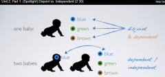
Week 02
Disjoint (Mutually Exclusive) vs Independent |
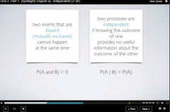
Note that with two indepdendent events P(A and B) = P(A) * P(B) |
|
|
Week 02
What is a contingency table? |
It is the table that can be drawn in lieu of a tree diagram. It also shows the distribution of one variable in rows and another in columns, used to study the association between the two. |
|
|
Week 02
What is a false negative? |
Rejecting as not positive when it should have been accepted as a true positive, such as a type II error which would yield a false negative. |
|
|
Week 01
What is a standardized score? |
It is another name for the z score. It's not called the s score to avoid confusion with the standard deviation.
|
|
|
Week 02
When an individual trial has only TWO possible outcomes, it is called a ______________ __________ _________. |
Bernoulli random variable. |
|
|
Week 02
Given that x% of the population of the group meet a criteria, what is the probability that in a random sample of y at least one y meets that criteria? |
One has to assume that none meet the criteria and take the complement. Mathematically, that is represented in the following way
1 - (1 - x/100) ^ y
1 - x/100 is the group that does not meet the criteria. When this value is raised to y. It is the probability that none of the sampled ones meet the criteria. Then subtracting it from 1 gives the result that at least one meet the criteria. |
|
|
Week 02
Describe the bernoulli distribution |
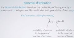
The binomial distribution describes the probability of having exactly k successes in n independent Bernouilli trials with probability of success p.
# of scenarios x P (single scenario)
See diagram left |
|
|
Week 02
Disjoint (Mutually Exclusive) vs Independent |
Note that with two independent events P(A and B) = P(A) * P(B) |
|
|
Week 02
Describe the equation for the binomial distribution |
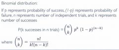
|
|
|
Week 02
What is a false negative? |
Rejecting as not positive when it should have been accepted as a true positive, such as a type II error which would yield a false negative.
Also, consider someone coming back as false negative on a test such as a drug screening. The person would, in reality, have the disease but come back negative on the test which is a false negative. |
|
|
Week 02
What is the difference between the dbinom, pbinom and binom.dist functions?
What are the order of the arguments for each? |
One is used with R and the other is used with excel; however, the results are the same (for pbinom and binom.dist( . . . cumulative=TRUE) and dbinom and binom.dist( . . . cumulative=FALSE) and each returns eihter a probability or density, respectively, based on the binomial distributions.
dbinom( # of successes, # of trials (size=x), probability (p=.13 (must be a decimal value where excel can take a decimal or percent))
binom.dist(# of successes, #of trials,probability(can be expressed as a %), cumulative (true of false))
|
|
|
Week 02
What is the expected value of a binomial distribution? |
Expected value is the mean, and it's simply the number of trials times the probability of success, that is,
mu = np
where n is the number of trials and p is the probability of success.
Example
Among a random sample of 100 employees, how many would you EXPECT to be engaged at work with a probability of success at .13
answer 100*.13 = 13 |
|
|
Week 02
What is the standard deviation for a binomail distribution? |
It is the square root of the mean times the probability of failure.
stddev = sqrt(np(1-p))
Example
Among a random sample of 100 employees, what is the standard deviation with a probability of success at .13
answer sqrt(100*.13*.87) = 3.36 |
|
|
Week 02
What is the success-failure rule for a binomial distribution?
Describe the conditions. |
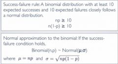
It allows us to use the known information about normal distribution to work with binomial distributions.
|
|
|
Week 02
What are the values for the following:
R Excel
|
Note, the combinations with 1 have a n result. The combinations without 1 show 1 as the result. |
|
|
Week 04
What is a running mean? |
A running mean is a sequence of means where the subsequent mean has one more observation than the previous mean.
Since point estimates such as a sample mean are usually not exactly equal to the truth, they get better as more data is added. |
|
|
Week 04
What is a sampling distribution? |
It is a collection of samples of fixed size of the same point estimate and thereby is called a distribution |
|
|
Week 02
What is the difference between the dbinom, pbinom and binom.dist functions?
What are the order of the arguments for each? |
One is used with R and the other is used with excel; however, the results are the same (for pbinom and binom.dist( . . . cumulative=TRUE) and dbinom and binom.dist( . . . cumulative=FALSE) and each returns either a probability or density, respectively, based on the binomial distributions.
dbinom( # of successes, # of trials (size=x), probability (p=.13 (must be a decimal value where excel can take a decimal or percent))
binom.dist(# of successes, #of trials,probability(can be expressed as a %), cumulative (true of false))
Cumulative Required. A logical value that determines the form of the function. If cumulative is TRUE, then BINOM.DIST returns the cumulative distribution function, which is the probability that there are at most number_s successes; if FALSE, it returns the probability mass function, which is the probability that there are number_s successes.
|
|
|
Week 04
The sample means of a distribution (sampling distribution) _________________ tend to "fall around" the population mean. |
should |
|
|
Week 02
What is the standard deviation for a binomial distribution? |
It is the square root of the mean times the probability of failure.
stddev = sqrt(np(1-p))
Example
Among a random sample of 100 employees, what is the standard deviation with a probability of success at .13
answer sqrt(100*.13*.87) = 3.36 |
|
|
Week 04
We use the standard error to identify what is ____________. |
close
pg. 164 OpenIntro Statistics |
|
|
Week 04
A range of values for the population parameter is called a confidence _____________ |
interval |
|
|
Week 04
Using _____________ a point estimate is like fishing in a murky lake with a spear, and using a confidene interval is like fishing with a __________. |
only, net |
|
|
Week 04
What does 95% confident mean? |
Suppose we took many samples and built a confidence interval from each same using the following:
point estimate +- 2 x SE
then about 95% of those intervals would contain the actual mean, mu, of the population
Also, it means that 95% of the time the estimate will be within 2 standard erros of the population parameter.
The 95% is taken from what we know about the characteristics of a normal distribution. |
|
|
Week 04 plau·si·bleˈplôzəb(ə)l/ |
(of an argument or statement) seeming reasonable or probable. |
|
|
Week 04
How does one start the derivation for Bayes' Theorem? |
Start with the general multiplication rule. |
|
|
Week 04
What is the informal definition for the CLT? |
IF a sample consists of at least 30 independent observations AND the data are not strongly skewed, then the distribution of the sample mean is well approximated by a normal model. |
|
|
Week 04
If X is a normally distributed random variable, how often will X be within 2.58 standard deviations of the mean? |
This is equivalent to asking how often the Z score will be larger than -2.58 but less than 2.58. To determine the look -2.58 and 2.58 in the normal probability table, use R or the online calculator to find 0.0049 and 0.9951, respectively. Therefore, there's a .9951-.0049 which is approximately .99 probaility that the unobserved random variable X will be within 2.58 standard deviations of mu. |
|
|
Week 04
How do we verify independence for the CLT? |
We keep the sample to less than 10% unless there's much skewness.
Observations in a simple random sample consisting of less than 10% of the population are independent. In other words, the chances of one observation having an impact on another is low. |
|
|
Week 04
Using _____________ a point estimate is like fishing in a murky lake with a spear, and using a confidence interval is like fishing with a __________. |
only, it leaves room for error |
|
|
Week 04
What does 95% confident mean? |
Suppose we took many samples and built a confidence interval from each sample using the following:
point estimate +- 2 x SE
then about 95% of those intervals would contain the actual mean, mu, of the population
Also, it means that 95% of the time the estimate will be within 2 standard erros of the population parameter.
The 95% is taken from what we know about the characteristics of a normal distribution. |
|
|
Week 04
Is the following correct or incorrect language when describing the confidence interval?
The confidence interval captures the population parameter with a certain probability. |
That is incorrect. The correct language is we are XX% confident that the population parameter is between . . . |
|
|
Week 04
An especially important consideration of confidence intervals is that they only try to capture the ___________________ parameter.
Our intervals say nothing about the confidence of capturing individual _____________, a _____________ of the observation, or about capturing a __________ __________ |
population, observations, proportion, point estimates |
|
|
Week 04
In RARE instances, we might know important characteristics of a population. Even so, we may still like to study __________________ of a random sample from the population. |
characteristics |
|
|
Week 04
If X is a normally distributed random variable, how often will X be within 2.58 standard deviations of the mean? |
This is equivalent to asking how often the Z score will be larger than -2.58 but less than 2.58. To determine the look -2.58 and 2.58 in the normal probability table, use R or the online calculator to find 0.0049 and 0.9951, respectively. Therefore, there's a .9951-.0049 which is approximately .99 probability that the unobserved random variable X will be within 2.58 standard deviations of mu. |
|
|
Week 04
If the null hypothesis is true, how often should the p-value be less than 0.05? |
Tricky question, the answer is about 5% of the time.
pg. 180 OpenIntro Statistics |
|
|
Week 04
What are the steps and how many are there in hypothesis testing using the normal model? |
1. WRITE the hypotheses in PLAIN LANGUAGE, then SET them UP in MATHEMATICAL NOTATION.
2. Identify an appropriate POINT ESTIMATE for the parameter of interest. 3. VERIFY CONDITIONS to ensure the POINT ESTIMATE is nearly NORMAL AND UNBIASED and the STANDARD ERROR ESTIMATE is REASONABLE. 4. COMPUTE the STANDARD ERROR. DRAW a picture depicting the distribution of the estimate UNDER THE IDEA THAT H-knot IS TRUE. SHADE AREA(S) REPRESENTING the p-VALUE. 5. Using the picture and normal model, COMPUTE the TEST STATISTIC (Z SCORE) and IDENTIFY the p-VALUE to EVALUATE HYPOTHESES. WRITE a CONCLUSION in PLAIN LANGUAGE. Note the test statistic is the observed data that supports the alternative hypothesis. |
|
|
Week 04
What does z* represent in the confidence interval? |
It represents the confidence LEVEL. Choose it in such a way that the area between -z* and z* in the normal model corresponds to the confidence interval. The higher z*, the higher the chance of capturing the sample statistic by the confidence interval. |
|
|
Week 04
Summarize the idea that is a p-value is < alpha then we reject the null hypothesis. |
When using determing the significance level, alpha, it is the same as setting the confidence level as for a confidence interval. Therefore, alpha, is setting a confidence interval, one or two-sided, where if it captures the test statistic, that is, it is within the bounds of the confidence interval set by alpha, then we fail to reject the null hypothesis.
Conversely, if the confidence interval set by alpha does not capture the test statistic, z*, then we say the evidence supports rejecting the the null hypothesis in favor of the alternative as it represents a rare event and the chances of that happening in one observation are slim. |
|
|
Week 04
Statistical tools rely on __________________. When the conditions are _________ met, these tools are unreliable and _____________ conclusions from them is ___________________. |
conditions, not, drawing, TREACHEROUS
|
|
|
Week 04
The conditions for basic statistical tools are: |
|
|
|
Week 04
We should _______________ state the conclusion of the hypothesis test in plain language so none statisticians can also understand the results. |
ALWAYS |
|
|
Week 04
Whenever conditions are not satisfied for a statistical technique, what options does one have to evaluate one's data? |
|
|
|
Week 04
The Type 2 Error rate and the magnitude of the error for a point estimate are controlled by the _____________ size. Real differences from the null value, even large ones, may be difficult to detect with ___________ samples. If we take a very large sample, we might find a statistically significant difference but the _____________ might be so small that it is of no practical value. |
sample, small, magnitude
|
|
|
Week 04
What is statistical significance? |
Woohoo, shout from the rafters, the status quo can be rejected, small p-value. (Can't "p"iss on one's "discovery parade"). The null hypothesis' assumption of true has a small p-value. Statistical significance is fundamental to statistical hypothesis testing.[11][12] In any experiment or observation that involves drawing a sample from a population, there is always the possibility that an observed effect would have occurred due to sampling erroralone.[13][14] But if the p-value is less than the significance level (e.g., p < 0.05), then an investigator may conclude that the observed effect actually reflects the characteristics of the population rather than just sampling error.[11] An investigator may then report that the result attains statistical significance, thereby rejecting the null hypothesis.[15] The present-day concept of statistical significance originated with Ronald Fisher when he developed statistical hypothesis testing based on p-values in the early 20th century.[2][16][17] It was Jerzy Neyman and Egon Pearson who later recommended that the significance level be set ahead of time, prior to any data collection.[18][19] |
|

Week 04
Who is Ronald Fisher? |
![Left, Fisher as a steward at the First International Eugenics Conference in 1912. Sir Ronald Aylmer Fisher FRS[2] (17 February 1890 – 29 July 1962) was an English statistician, evolutionary biologist, mathematician, geneticist, and eu...](https://images.cram.com/images/upload-flashcards/98/57/96/9985796_m.jpg)
Left, Fisher as a steward at the First International Eugenics Conference in 1912.
Sir Ronald Aylmer Fisher FRS[2] (17 February 1890 – 29 July 1962) was an English statistician, evolutionary biologist, mathematician, geneticist, and eugenicist. Fisher is known as one of the chief architects of the neo-Darwinian synthesis, for his important contributions to statistics, including the analysis of variance (ANOVA), method of maximum likelihood, fiducial inference, and the derivation of various sampling distributions, and for being one of the three principal founders of population genetics. Anders Hald called him "a genius who almost single-handedly created the foundations for modern statistical science",[3] while Richard Dawkins named him "the greatest biologist since Darwin" |
|
Week 01
Who is Thomas Bayes? |
Thomas Bayes (/ˈbeɪz/; c. 1701 – 7 April 1761)[1][2][note a] was an English statistician, philosopher and Presbyterian minister, known for having formulated a specific case of the theorem that bears his name: Bayes' theorem. Bayes never published what would eventually become his most famous accomplishment; his notes were edited and published after his death by Richard Price.[3]
Thomas Bayes was the son of London Presbyterian minister Joshua Bayes,[4] and was possibly born in Hertfordshire.[5] He came from a prominent nonconformist family from Sheffield. In 1719, he enrolled at the University of Edinburgh to study logic and theology. On his return around 1722, he assisted his father at the latter's chapel in London before moving to Tunbridge Wells, Kent, around 1734. There he was minister of the Mount Sion chapel, until 1752.[6]He is known to have published two works in his lifetime, one theological and one mathematical:Divine Benevolence, or an Attempt to Prove That the Principal End of the Divine Providence and Government is the Happiness of His Creatures (1731)An Introduction to the Doctrine of Fluxions, and a Defence of the Mathematicians Against the Objections of the Author of The Analyst (published anonymously in 1736), in which he defended the logical foundation of Isaac Newton's calculus ("fluxions") against the criticism of George Berkeley, author of The AnalystIt is speculated that Bayes was elected as a Fellow of the Royal Society in 1742[7] on the strength of the Introduction to the Doctrine of Fluxions, as he is not known to have published any other mathematical works during his lifetime.In his later years he took a deep interest in probability. Professor Stephen Stigler, historian of statistical science, thinks that Bayes became interested in the subject while reviewing a work written in 1755 by Thomas Simpson,[8] but George Alfred Barnard thinks he learned mathematics and probability from a book by Abraham de Moivre.[9] His work and findings on probability theory were passed in manuscript form to his friend Richard Price after his death.Monument to members of the Bayes and Cotton families, including Thomas Bayes and his father Joshua, in Bunhill Fields burial ground. By 1755 he was ill and by 1761 had died in Tunbridge Wells. He was buried in Bunhill Fields burial ground in Moorgate, London, where many nonconformists lie. |
|

Who is Gottried Achenwall?
|
![Gottfried Achenwall (20 October 1719 – 1 May 1772) was a German philosopher, historian, economist, jurist and statistician. He is counted among the inventors of statistics.
Biography
Achenwall was born in Elbing (Elbląg[1][2]) in ...](https://images.cram.com/images/upload-flashcards/98/66/72/9986672_m.jpg)
Gottfried Achenwall (20 October 1719 – 1 May 1772) was a German philosopher, historian, economist, jurist and statistician. He is counted among the inventors of statistics.
Biography Achenwall was born in Elbing (Elbląg[1][2]) in the Polish province of Royal Prussia.[3] Beginning in 1738 he studied in the Jena, Halle, again Jena and Leipzig. In the years 1743 to 1746, he worked as controller in Dresden. He was awarded his master's degree in 1746 by the philosophical faculty of Leipzig and went in the following to Marburg to work as assistant professor lecturing history, statistics, natural and international law. In 1748 he was called to the University of Göttingen to become extraordinary professor of philosophy, and in 1753 he became an extraordinary professor of law and regular professor of philosophy. In 1761 he again shifted fields, becoming a professor of natural law and politics, and in 1762 he became a doctor of both laws.In 1765, Achenwall became court counsellor of the Royal British and the Electoral court of Hanover. With financial support from King George III he travelled to Switzerland and France in 1751 and to Holland and England in 1759. He died in Göttingen, aged 52.In economics, he belonged to the school of “moderate mercantilists”; but it is in statistics that he holds his greatest renown. The work by which he is best known is his Staatsverfassung der Europäischen Reiche im Grundrisse (Constitution of the Present Leading European States, 1752). In this work, he gave a comprehensive view of the constitutions of the various countries, described the condition of their agriculture, manufactures and commerce, and frequently supplied statistics in relation to these subjects. German economists claimed for him the title of “Father of Statistics”; but English writers disputed this, asserting that it ignored the prior claims of William Petty and other earlier writers on the subject. Achenwall gave currency to the term Staatswissenschaft (politics), which he proposed should mean all the knowledge necessary to statecraft or statesmanship.[4] |
|

Who is Sir William Petty?
|

Sir William Petty FRS (26 May 1623 – 16 December 1687) was an English economist, scientist and philosopher. He first became prominent serving Oliver Cromwell and Commonwealth in Ireland. He developed efficient methods to survey the land that was to be confiscated and given to Cromwell's soldiers. He also managed to remain prominent under King Charles II and King James II, as did many others who had served Cromwell.He was Member of the Parliament of England briefly and was also a scientist, inventor, and entrepreneur, and was a charter member of the Royal Society. It is for his theories on economics and his methods of political arithmetic that he is best remembered, however, and to him is attributed the philosophy of 'laissez-faire' in relation to government activity. He was knighted in 1661. He was the great-grandfather of Prime Minister William Petty Fitzmaurice, 2nd Earl of Shelburne and 1st Marquess of Lansdowne.
|
|
|
Week 04 |
It would be reasonable to review scientific literature or market research to make an educated guess about the standard deviation.
|
|
|
Week 04
Sample size computations are helpful in _______________ data collection, and they require _______________ forethought. What is another important topic in planning data collection and setting sample size? |
planning, careful
the Type 2 Error rate |
|
|
Week 04
What is the mathematical notation to represent a normal distribution with mean, mu, μ, and, standard deviation, sigma, σ? |
N ( μ,σ )
|
|
|
Week 04
What are the z-scores associated with the following confidence intervals?
|
Find the z-score (standard deviations from the mean) by
|
|
|
Week 04
What should this value not be confused with? |
power.
This should not be confused with alpha, which the probability of making a Type 1 error, that is, incorrectly rejecting the null hypothesis. |
|
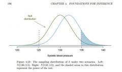
Week 04
The _________ varies depending on what we suppose the truth might be. In other words. The power _______ depending on how far from the truth we are. If the distance (value) from the truth is small, then the power will be __________ . The two are _______________ proportional. Another way of looking at power, is the smaller the difference between the actually truth and the supposed truth, the more ____________ it is to see the difference between the two. When the sample size become larger, point estimates become more precise (implied by the standard error equation) and any real ___________ in the mean and null value become ____________ to detect and recognize. Sometimes researchers will take such large samples that even the slightest difference is ________________. |
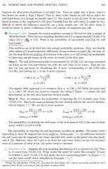
power small, directly difficult differences, easier detected |
|
|
Week 04
What is the difference between statistical significance and practical significance? |
Practical significance is statistical significance but the converse is not necessarily true.
Statistical significance provides statistical evidence to support the alternative hypothesis; however, it may not have real world application, thereby, being a waste of time and money to arrive at the result. We don't want to spend lots of money finding relts that have no practical value. |
|
|
Week 04
The role of a statistician in conducting a study often includes __________ the size of the study. The statisticain might first consult experts or scientific ___________________ to learn what would be the _______________ meaningful difference from the null value. |
planning, literature, smallest
|
|

Week 04
Provide an intuitive explanation for why we are more likely to reject H-knot when the true mean is further from the null value? |

When the point estimate is calculated based on the alpha that is set prior to collecting data, the point estimate, assuming all conditions are met and little to no sampling biases exist, it will capture the mean at the level set by the z-score. Therefore, considering the graph at left, the more the blue (truth) mean moves a way from the null's mean their overlap become smaller and smaller. Similar to a Venn Diagram, that translates into fewer and fewer "shared" values which means a lower probability of both having the same values overlapping and this is where the true mean would have to lie.
|
|

Week 04
If the power of a test is .979 for a particular mean, what is the Type 2 Error rate for this mean? |

It is the complement of the power test, that is, 1-.979 = .021, very low, which is ideal if favoring the alternative hypothesis.
|
|

Week 04
The type 2 Error rate represents the probability of failing to reject the null hypothesis then the power is the probability of not failing to reject the null hypothesis since the two are ________________. What is another way of saying "not failing to reject the null hypothesis"? |

compliments
we do reject |
|
|
Week 05
TWO set of observations are paired if each observation in one set has a special __________________ or ___________________ with exactly __________ observation in the other data set |
correspondence, connection, one
|
|
|
Week 05
Although the experiment in Chapter 4 of OpenIntro Statistics took a difference of a control group and treatement group to determine the effect of a drug on the death rate on heart attack patients and the point estimate was determined by taking the difference in the two, this data does _________ comprise paired ___________ since there is no _________ correspondence or connection between the control group and treatment groups. That is, the groups are look as a whole instead of individual parts that are compared and then used to calculate descriptive statistics. |
not, data, SPECIAL.
This could be said for any mean under probability theory where the alternative hypothesis is established where it is a two-tailed test. That is, attempting to show there is no difference between the point estimate and the population mean. |
|
|
Week 05
To analyze paired data, we use the ____________ same tools that we learned in hypothesis testing (Week 04) |
exact
|
|
|
Week 05 Inference for Numerical Data, Paired Data
The ____ difference scenario is _________ the null hypothesis. |
no, ALWAYS
|
|
|
Week 05
T or F The conditions (Central Limit Theorem) on which the normal model can be used must be reasonably met as opposed to absolutely met. T or F If the conditions are reasonable, the point estimates will be reasonable. |
True, true.
|
|
|
Week 05
Is the difference of two means the same as paired data? |
Not necessarily, paired data will be the difference in two means; however, the difference in two means may not be paired data. For instance, if one were to consider the birth weights of new borns to mother's who smoke vs. mother's who do not smoke, there's no relationship other than the consideration of the weight of the newborn.
On the contrary, if one were to consider the price of a book that is offered through two different retailers like the Univ of Cal, Berkeley or Amazon, the same book is being considered. |
|
|
Week 05
If two samples are independent of one another, then they are not ______________. |
paired.
This is an important concept as the data inside the samplings could be independent and for the scope of this online course will be independent but they are not paired because across the data sets, they are independent. |
|
|
Week 05
What is the conditon formality of x1(bar) - x2(bar), non-paired? |
If the sample means, x1(bar) - x2(bar), each meet the criteria for having nearly normal sampling distributions and the observations in the two samples are independent, then the difference in sample means, x1(bar)-x2(bar) will have a sampling distribution that is nearly normal.
|
|
|
Week 05
What is the formula for two sample means' standard error? |
SE( x1(bar)-x2(bar) ) =
sqrt( var1(bar)/sampsize1(bar) + var2(bar) + sampsize2(bar) ). Observation, the fact that variance as opposed to stddev is used in this formula complicates it. Otherwise, it looks similar to the standard error for a single mean. Also, the standard deviation means can be used since typically the standard deviation of the population is not KNOWN. We like knowns. :-) Take advantage of that to memorize it. |
|
|
Week 05
Probability theory ______________ that the difference of two independent normal random variables is also ___________________. |
guarantees, normal.
|
|
|
Week 05
Yes or No. Is calculation the confidence interval for the difference in two independent random variables different than what we no about a single random variable. |
No. It's simply the point estimate plus or minus the z-score times the standard error.
|
|
|
Week 05
What does 95% confidence mean? |
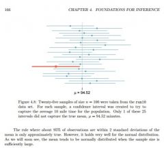
It means if we were to collect many such samples and create 95% confidence intervals for each, then about 95% of those intervals would contain the mean, which could be the difference in two random independent means.
See example from Week 04 left. |
|
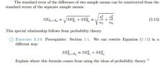
Explain where the formula, left, in Exercise 5.14 comes from.
|
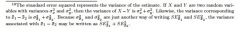
|
|
|
Week 05
What two consequences are a result of a large sample size for a normal distribution that are not necessary for a t distribution? |
|
|
|
Week 05
The __ distribution is a helpful substitute for the normal distribution when modeling a sample mean that comes from a small sample. While it is stressed that a t distribution be used with small samples, it can also be used for means from ____________ samples. |
t, large
|
|
|
Week 05
How is the CLT for NORMAL DATA different from the CLT for any data? What is a drawback of CLT for NORMAL DATA? |
The CLT for NORMAL DATA is a condition that must exist when using small samples as for those used along with the t distribution and states that the data must be independent and come from a distribution that is nearly normal. Therefore, the data cannot be skewed which the CLT accounts for by allowing the researcher to take a larger sample size.
It's inherently difficult to verify normality in small data sets. Taking a larger sample size may not be possible. Hence, the data with small sample must be nearly normal. |
|
|
Week 05
Considering the CLT for NORMAL DATA, we should exercise caution when verifying normality condition for __________ sample sizes. It's important to not only ___________ the data but also think about from ___________ it came. LOL :-) |
small, analyze, whence
|
|
|
Week 05
With the CLT for NORMAL DATA, one may __________ the normality condition as sample size increases. If the sample size is __________ or more, slight skew is not problematic. Once the sample size hits about ______, then moderate skew is reasonable. Data with ____________ skew or ___________ require a more cautious analysis. |
relax, 10, 30
strong, outliers |
|
|
Week 05
Visually, how does a t distribution differ from a normal distribution? |
It has fatter (thicker) tails which more observations ARE LIKELY to fall beyond two standard deviations.
|
|
|
Week 05
The fatter (thicker) tails of of the t distribution are __________ what are needed to resolve the _________ associated with the poor estimate of the standard error for small samples. |
exactly, problem
|
|
|
Week 05
T or F. The t distribution is always centered at zero. |
True
|
|
|
Week 05
T or F. The t distribution has a single parameter. |
T, it's called the degrees of freedom (df).
|
|
|
Week 05
In a t distribution, what function does the df have? |
It describes the form of the bell-shaped distribution.
|
|
|
Week 05
T or F Different from a normal distribution, the t distribution actually has a standard deviation of a little more than one? Does this makes sense? Explain. |
T, it makes sense since the tails are thicker than that of a normal distribution which means one has to move further from the mean to capture 68% of the distribution.
Note for all of the applications associated with this OpenIntro Statistics, it thinks of the t distribution as have a standard deviation of 1. |
|
|
Week 05
How do the df's of a t distribution relate to that of a normal distribution? |
The higher the df of a t distribution then the more the distribution looks like a normal distribution.
Imagine squeezing the tails to "push" more of the distribution toward the mean, that is, flatten the tails. So, the higher the df the flatter (thinner) the tails. |
|
|
Week 05
What df makes a t distribution almost indistinguishable from a normal distribution? |
30
|
|
|
Week 05
What table is used for t distibutions in lieu of the normal probability table used for normal distributions? |
Let me see? The t table, good guess.
|
|
|
Week 05
Describe the t table? |
Each row represents a t distribution with different df, and the columns correspond to the tail probabilities. So, different from a normal probability table, the columns (labels) of the table represent probabilites instead of the center of the table.
The center's represent the "t-score" (standard deviations from the mean) or "cutoffs" so it's reversed from a normal probability table. Also, note for a t score, the probability represents the area to the right of the tail, and, if a probability is needed for an observation that falls below the mean, take the absolute value of that t-score and read the corresponding probabilty. It will be the same as the negative t-score value. |
|
|
Week 05
How does one calculate the degrees of freedom for a single sample? |
It is df = n - 1 where n is the sample size
|
|
|
Week 05
What is t*and how is it determined? |
It is the multiplication factor and represents the number of standard deviations from the mean. It is found by entering the t table with two known variables. They are the df and the desired confidence interval. With these two variables, one can locate t* at the center of the table where the known variables intersect.
Note two variables are required to determine t* (df and probability) where as only one variable (probability) was necessary for z*. |
|
|
Week 05
What is the formula for constructing a confidence interval for a t distribution? |
It's similar to that of a normal distribution,
x(bar) +- t*(df) * SE t* is a function of two variables, df and the probability of it's occurrence. |
|
|
Week 05
What is the difference in z* and t* and z test statistic and t test statistic, respectively? |
z* and t* are similar in that each starts with a confidence interval which is the probability needed based on alpha to capture the population parameter.
The alpha, once determined, is compared to the p-value since both are probabilities. Remember; alpha is the compliment of the confidence interval and the probability one uses to compare to the p-value (another probability) derived from the test statistic computed using the observation. z test statistic and t test statistic start with a point estimate and these values are calculated from which the probability can be determined. Thinking about the distribution tables of z* and t*, one uses the distribution, and, in the case of a t distribution, the degrees of freedom to locate the probability needed. In most cases, this is the p-value or the p-value's compliment from which the p-value can be calculated. From the distribution tables or a distribution calculator, one can work backwards to find the z-score or t-score. Again and in contrast, on the other hand one starts with a point estimate and finds the test stastic to determine the probability (p-value) of the occurence of the point estimate. Note the test statistic is more involved because one has to compute it and then use it to get the probability as opposed to being given the probability from the significance level and then looking up the "distribution score", quantile or cutoff value or using software to determine it. |
|
|
Week 05
Described how a confidence interval can be constructed after rejection of H(knot), the null hypothesis, due to a small p-value to show that the true value lies somewhere between the interval? |
Considering Exercise 5.33, pg 235, embryonic stem cells were shown to provide convincing evidence that they improve heart pumping function so the null hypothesis was rejected. Based on that inference, the confidence interval can be constructed using the point estimate, the z or t score for the desired confidence interval, and the SE.
Note, prior to the test the confidence interval being tested to see if it contains the p-value was based on the assumed to be true mean. Once it's rejected, one can construct the true confidence interval, using the point estimate as described above. |
|
|
Week 05 (Special Topic)
T or F Two populatons will occasionally have standard deviations that are so similar that they can be treated as identical. |
T. This is how we arrived at POOLED standard deviations.
|
|
|
Week 05 (Special Topic)
What are pooled standard deviations? |
It is a WAY to use data from samples with identical, for all practical purposes, standard deviations to arrive at better estimates for the standard deviation and standard errors.
|
|
|
Week 05 (Special Topic)
What is the formula for pooled standard deviations. |
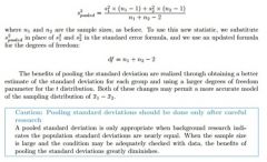
|
|
|
Week 05
Describe a way of comparing three means? What is a more efficient method and what is it called? |
Compare 1 and 2
Compare 1 and 3 Compare 2 and 3 ANOVA is a more efficient method as it allows us to compare several means with one hypothesis test as opposed to three as shown above? |
|
|
Week 05
What is the basis for setting up the hypothesis to be evaluated using ANOVA? |
H(null) - all the hypothesis are equal. Another way of saying this is, there is no difference which is what we've used up to the point.
H(alternative) - there is a difference OF AT LEAST ONE MEAN. |
|
|
Week 05
What are the conditions for ANOVA? |
There are generally three conditions
|
|
|
Week 05
What is data snooping or data fishing? Based on these ideas what is the prosecutor's fallacy? |
Inappropriately, it is examining all data by ey (informal testing) and only aferwards deciding which parts to formally test. :-(
The prosecutor's fallacy is a fallacy of statistical reasoning, typically used by the prosecution to argue for the guilt of a defendant during a criminal trial. |
|
|
Week 05
What is the gambler's fallacy? |
The gambler's fallacy, also known as the Monte Carlo fallacy or the fallacy of the maturity of chances, is the mistaken belief that, if something happens more frequently than normal during some period, it will happen less frequently in the future, or that, if something happens less frequently than normal during some period, it will happen more frequently in the future (presumably as a means of balancing nature).
In situations where what is being observed is truly random (i.e., independent trials of a random process), this belief, though appealing to the human mind, is false. This fallacy can arise in many practical situations although it is most strongly associated with gambling where such mistakes are common among players. |
|
|
Week 05
What is the mean square between groups? |
The variability in the sample means in a group of means being evaluated using ANOVA.
|
|
|
Week 05
With the method of analysis of variance used in OpenIntro Statistics, what is the one question that is the focus of our hypothesis testing? |
Is the variability in the sample means so large that it seems unlikely to be from chance?
|
|
|
Week 05 |
Mean Square Groups. It is associated with ANOVA analysis?
|
|
|
Week 05
How does one calculate the associated degrees of freedom for MSG? |
By using the following formula?
df(G) = k -1 where k is the number of groups being analyzed. |
|
|
Week 05
T or F The MSG on its own is quite useless. Why or Why not? |
This true. There has to be a benchmark for what variability should be expected among the sample means if the null is true to which it can be compared.
|
|
|
Week 05
What does MSE stand for and how is it used? |
It is the mean square error, and its used in combination with MSG as a point of comparison in determining what the expected variability should be among the groups' sample means.
|
|
|
Week 05
What is the associated degrees of freedom for the MSE? |
It is df(E) = n-k, where n is the sample size of the groups.
|
|
|
Week 05
Conceptually, how should one interpret MSE? |
It is the variability within the groups.
|
|
|
Week 05
What is the formula for the F statistic? Interpret it components. |
F = MSG/MSE where MSG is variability across groups and MSE is variability within groups.
This is in line with other scores such as t and z as they are a measure of variability too based on standard deviations when the SE is expressed in terms of variability from the mean. Note that SE is contained in the denominator of the F score as well. Also, note is variability is the same the F-statistic will be one. |
|
|
Week 05
How does one calculate the p-value for an F distribution? |
Using two known parameters, df(1) = df(G) and df(2) = df(E)
|
|
|
Week 05
T or F The larger the observed variability in the sample means (MSG) relative to the within-group observations (MSE) , the larger the F will be and the stronger the evidence against the null hypothesis. How is this consistent with other test statistics? |
T. This is consistent with other tests statistics as the bigger the test statistics, the more representative they are of moving away from the null hypothesis, increasing the likelyhood of not being observed based on an assumed to be true null hypothesis.
|
|
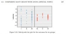
Week 05
Explain this diagram as it relates to the requirement for variance within groups to be similar with using ANOVA. |
It is a visual of how these set of data do not conform to the third condition of ANOVA where the data within the groups must have similar variances, that is, the spread from top to bottom must be close. The subgroup of 4, 5 and 6 would meet the requirement. However, looking at the group as a whole would not. |
|
|
Week 05
In ANOVA analysis, when we reject the null hypothesis, how do we determine which means have a difference present? |
We refer back to what we initially stated what the researcher should not do, that is, data snooping or data fishing.
We also go against the idea of using ANOVA where we compare the identified data where differences might exist such in mean 1, 2, and 3. We would then do a combin(3,1). |
|
|
Week 05
What is "muliple comparisons"? |
It is the scenario of comparing many pairs of groups as might be done after rejecting the H-knot(null) using ANOVA to determine among which groups do a difference in means lie.
|
|
|
Week 05 |
It is used with testing two samples using a t distribution for differences after rejecting the null hypothesis using ANOVA where we use a more stringent significance level by cutting it into pieces based on the number of groups (k).
It is used to avoid increasing the type 1 error rate after doing multiple tests. The equation is alpha(*) = a/K where alpha is the significance level and K is the number of comparisons being considedered. If there are K groups, then usually all possible pairs are compared and K = k(k-1)/2 or combin (K,2) = K!/(2!(K-2)!=k(k-1)/2 |
|
|
Week 05
Using a Wall Street analogy, describe how use of ANOVA may lead one to reject the null but not be able to find differences between any two means. |
We observe a Wall Street firm that makes larege quantities of money based on predicting mergers. Mergers are generally difficult to predict, and if the prediction sucees rate is extremely high, that may be considered sufficiently strong evidence to warrant investigation by the SEC.
While the SEC amy be quite certain that there is insider trading taking place at the firm, the evidence against any single trader may not be very strong. It is only when the SEC considers all the dat that they identify the patter. This is effectivley the strategy of ANOVA; stnad back and conside all the groups simultaneously. |
|
|
Week 05
What is the compliment of the significance level? |
The confidence level. Do not confuse this with the confidence interval, although the numerical representations are the same, the confidence interval is a visual representation of where the null hypothesis will lie if true.
|
|
|
Week 05
What are side by side box plots good for? |
They are good for a visual representation of a categorical variable combined with a numerical variable.
|
|
|
Week 05
When would the median as opposed to the mean be a better estimate of a "midpoint" of a set of data? |
When the data is skewed.
|
|
|
Week 01
What is a statistic? |
A FACT or PIECE OF DATA from a study of a large quantiy of numerical data. (Source: Google)
A SINGLE measure of some ATTRIBUTE of a sample, e.g. its arithmetic mean value. (Source: Wikipedia) |
|
|
What is the z distribution?
|
It is the proverbial normal distribtion, different from a t distribution.
|
|
|
Week 05
What is another name for quantiles? |
cutoff values.
|
|
|
Week 05 What should one do prior to determining the p-value? |
Draw a picture with the cutoff values, that is, the test statistic or quantiles.
|
|
|
Week 05
With the t distribution, more degrees of freedom _______________ to more data. |
equates.
Think about the equation for df(t) and how this makes sense. Also, will the higher the degrees of freedom the more the shape of the t-distribution approaches the z distribution (normal distribution) |
|
|
Week 01
In R, what does lower.tail mean? |
This means the tail portion left of the specified quantile or cutoff, that is, the statistic score or test statistic.
|
|
|
Week 01
R returns a probability that is left of the statistic score (for example, z score), how would one go about getting the probability to the right of the statistic score? |
specify that the lower.tail = FALSE which will yield the probability that is right of the statistic score.
|
|
|
Week 01
Using R how would one get a value for a two-tail test statistic? |
make the lower.tail = FALSE and multiply by 2. This can be done in the R console for instance the following t test statistic would yield a two tailed probability
> 2*pt(2.24,21,lower.tail=FALSE) where 2.24 is the t test statistic and 21 is the degrees of freedom REMEMBER R is case-sensitive, different from VB |
|
|
Week 01
Is R case-sensitive? How does this differ from VB? |
Yes, it is. VB is not case sensitive.
|
|
|
Week 06 Inference for Categorical Data
A sample proportion from a __________ variable can be defined as a sample _________ |
categorical, mean
|
|
|
Week 06 Inference for Categorical Data
When certain _____________ are met, a ___________ proportion is well characterized by a ____________ distribution. |
conditions, sample, normal
|
|
|
Week 06 Inference for Categorical Data
In a sample proportion, if we represent each "success" as a 1 and each "failure" as a 0, then describe describe the mathematical formula for calculating its mean. |
p(hat) = 0+1+1+ . . . +0 / the number of outcomes.
|
|
|
Week 06 Inference for Categorical Data
The distribution of p(hat) is nearly normal when the distribution of 0's and 1's is not too strongly ______________ for the sample size. |
skewed
|
|
|
Week 06 Inference for Categorical Data
What is the most common guideline for skew and size of the sample when working with proportions? |
One should expect to observe a minimum number of successes and failures, typicallay at least 10 of each.
|
|
|
Week 06 Inference for Categorical Data
What are the conditions for the sampling distribution of p-hat to be nearly normal and how do they compare to the CLT? |
The sampling distribution for p(hat), taken from a sample of size n from a population with a true proportion p, is nearly normal when
In comparison, the central limit theorem (CLT) states that, GIVEN CERTAIN CONDITIONS, the arithmetic mean of a sufficiently large number of iterates of independent random variables, each with a well-defined expected value and well-defined variance, WILL BE APPROXIMATELY normally distributed. So, they both discuss independence of the observations and size of the sample (sufficiently large for a normal distribution and the success-failure condition for p-hat). |
|
|
Week 06
Name and describe the distributions learned up to this point |
BGB NPN t |
|
|
Week 06
What is the formula for the standard error for a sample proportion? |
The standard error is SE(p(hat)) =
sqrt(p(1-p)/n) or for ease of memorization in making it look more like the SE for a normal (z) distribution sqrt(p(1-p))/sqrt(n) |
|
|
Week 01
What is a summary statistic? |
A summary statistic is a single number summarizing a large amount of data.
|
|
|
Week 01
The standard deviation is useful when _______________ how close the data are to the mean. |
considering
|
|
|
Week 01
What is an outlier? |
It's an observation that seems extreme relative to the rest of the data.
|
|
|
Week 01
Why is it important to look for outliers? |
|
|
|
Week 01
What are robust estimates? |
When extreme observations has little affect on the estimates value such as a median, mean, or IQR.
|
|
|
Week 01
What is another name for expected value? |
The mean.
|
|
|
Week 01
Do not confuse an observation's deviation (z-score) with the ________________ or the point estimate's standard deviation |
population's
|
|
|
Week 01
Can we determine what type of distribution we are dealing with by looking at a population's mean and standard deviation values? |
No. Think about the CLT for a normal (z) distribution which imposes conditions to have a data set conform to the z distribution so the data can be evaluated.
Also, typically these values are not known but we know if we apply certains conditions the sample data will fit into a certain type of distribution from which then we can test the data to establish inferences, given we apply the conditions. In spite of the above, given a data set has a normal distribution then we know that the 68%, 95%, 99.7% rule applies. |
|
|
Week 01
What is standard deviation according to Investopedia? Conceptually, what does it represent? |
A measure of the dispersion of a set of data from its mean.
Conceptually, the more spread apart the data, the higher the deviation. Standard deviation is calculated as the square root of variance. INVESTOPEDIA EXPLAINS 'Standard Deviation'Standard deviation is a statistical measurement that sheds light on historical volatility. For example, a volatile stock will have a high standard deviation while the deviation of a stable blue chip stock will be lower. A large dispersion tells us how much the return on the fund is deviating from the expected normal returns.Read more: http://www.investopedia.com/terms/s/standarddeviation.asp#ixzz3XG2O2B4F Follow us: @Investopedia on Twitter |
|
|
Week 06
No estimate of the ______ proportion is required in sample size computations for a proportion whereas an estimate of the _____________ ___________ is ALWAYS needed when comptuing a sample size for a margin of error for the sample mean. T or F However, if we have an estimate of the proportion, we should use it in place of the worst case estimate of the proportion, 0.5 |
true, standard deviation
T |
|
|
Week 06
What are the conditions for the sampling distribution of p(1)hat - p(2)hat to be normal? |
The difference p(1)hat - p(2)hat tends to follow a normal model when
|
|
|
Week 06
What is the standard error of the difference in sample proportions. |
It looks very similar to the standard error for two sample means in that one adds the two variances after dividing each by its respective sample size then take the square root of the result ___________ ___________________ √ SE2p̂1 +SE2p̂2 = √ p1(1- p1)/n1 + p2(1- p2)/n2 |
|
|
Week 06
standardize as the standard error or standard deviation |
(cause) something to conform to a standard.
|
|
|
Week 06
The _______________ distribution is sometimes used to characterize data dets and statistics that are _______________ positive and typically ___________ skewed. |
chi-square, ALWAYS, right
|
|
|
Week 06
What are the parameters of the chi-square distribution? And what do they affect. Recall; what are the parameters of a normal distribution? |
This is a trick question. The chi-square distribution has just one parameter, that is, df.
The df influences the
They're the mean and standard deviation. |
|
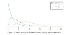
Week 06
The figure at left shows three chi-square distributions. How does the center of the distribution change when the df is larger? What about the variability (spread or dispersion)? How does the shape change? |
In general, as df increases, the distribution flattens
Specifically,
|
|
|
Week 06
What table does one use for the chi-square distribution? What table is it similar to? What are the differences between the table? |
The chi-square table
It is similar to the t distribution table as the rows for both are defined by the df. There is one difference, that is, the column for the t table defines the left or right ( or lower and upper) tail, and the columns for the chi-square just defines the upper tail since all values are positive and the distribution is skewed right, generally with low df. |
|
|
Week 06
How does one determine the df with chi and what does it represent? |
It is k-1, where k represents the number of bins
|
|
|
Week 06
Describe the chi-square for a one-way table? |
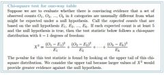
|
|
|
Week 06
What are the conditions for the chi-square test? |
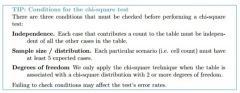
|
|
|
Week 06
What sections of OpenIntro Statistics discuss determining "goodness of fit" of a set of data to a distribution? |
Sections 3.3 and 6.3
|
|
|
Week 06
Ephipany: The expected values tell us what the ______________ (null hypothesis) should predict. The observe values are the _____________ and the good news is we can test (alternative hypothesis) them with a ___________ _____________ that corresponds to the truth (observed value). |
model, truth, test statistic
|
|
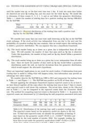
Week 06
Describe the test at left at the conclusion |
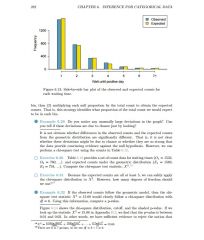
|
|

Week 06
What is so different about one-way tables and two-way tables such as the two-way table left involving a Google experiment? |
A one-way table describes counts for each outcome in a single variable. A two-way table describes counts for comvinations of outcomes for two variables.
When we consider a two-way table, we often would like to know, are thes variables related in any way? That is, are they dependent (vs. independent)? |
|
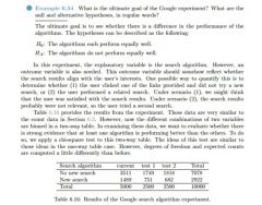
Week 06 |
it is
Expected Count (row i, col j) = (row i total) x (column j total) / table total Conceptually, this formula yields a percentage (probability of the total column or total row occurring) and the resulting value is multiplied by the remaining total column or total row, the value that was not used to compute the percentage (probability) |
|
|
Week 06
How is the chi-square test for a two-way table computed? |
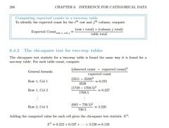
It is found the say way it is found for a one-way table.
The general formula is (observed count - expected count)^2/expected count Notice how the numerator for this formula look similar to that for the z-score, in that, it is the obs - expected. The difference is it is squared which always yields a positive value. Additionally, notice how it is "standardized" in terms of the expected value since the denominator is the expected value. In other words, the resulting value is expressed in terms of the expected value. Note this formula has to be used iteratively for each observation. The iterations are them summed to arrive at the test static. |
|
|
Week 06
How does one compute df for a two-way table whose data conforms to a chi-distribution? |
df = (R-1) x (C-1)
where R is the number of rows and C is the number of columns in the table. Recall that in a one-way table, the df is the number of cells (columns or categories) minus 1 |
|
|
Week 06
When using the one-sided hypothesis test for p with a small sample, what problem does this present and how does one overcome that? |
The p-value is always derived by analyzing the null distribution of the test statistic. The normal model poorly approximates the null distribution for p-hat when the success-failure condition is not satisfied. As a substitue, we can generate the null distribution using simulated sample proportions, p-hat(sim), and use this distribution to compute the tail area, i.e. the p-value
|
|
|
Week 06
The chi-square distribution has similarities to a binomial distribution, in that, it is binary. Explain the attributes that separate the two. |
The chi-square distribution deals with categorical variables, and even though, it can be represented numerically for hypothesis testing, the numerical characteristics describing data on deal with frequency of the data and a categories success-fail rate.
This idea needs more in depth studying of the binomial distribution as it appears to have the same characteristic. Remember, binomial distributions deal with success and failures as well. In chi-square, we determine dependence or independence |
|
|
Week 06
Describe the extent of categorical variables that are used in OpenIntro Statistics? |
One (1) categorical variable
Two (2) categorical variables
|
|
|
Week 06
If the sample is a categorical variable, then the sample statistic is a ______________________. |
proportion (ratio)
|
|

Week 06
Graphically describe the difference between a sample distribution and a sampling distribution? |
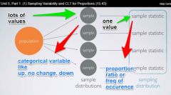
One starts with the population. From there, sample are taken, in this case, a variable that is categorical. The collection of samples represents the sample distribution. The sample is represented by a proportion (ratio). The collection of proportions represent the sampling distribution.
Note: The sample distribution could be people or something other than a numerical value whereas the sampling distribution will be a statistic. |
|
|
Week 06
What does p-hat ~ N? |
It means the sample proportion will be NEARLY (~) normal.
|
|
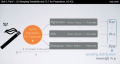
Week 06
Describe how the problem at left, although calculated using proportions as shown, could be solved using the binomial distribution. |

Notice how 190 successes constitute the number of successes.
Also, note with sum and a range 190:200 these values are added up to arrive at the probability. The equivalent function is excel is BINOM.DIST.RANGE(200,.9,190,200) |
|
|
Week 06
What is the success-failure condition is not met when testing conditions to see if data conform to a proportion? |
|
|
|
Week 06
T or F A sampling distribution of a proportion must be between 0 and 1 |
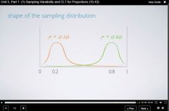
True because all proportions are positive.
|
|
|
Week 06
What would you expect the shape of the sampling distribution of percentages of angiosperms (flowering plants) in random samples of 50 plants to look like? (Remember, 90% of all plants species are classified as angiosperms? |
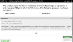
left skewed
|
|
|
Week 06
The confidence level is about percentage of _______________ that yield intervals capturing the ___________ parameter, not about predicting where _________ samples will fail. |
samples, population, future.
|
|
|
Week 06
When do we use p-hat (sample statistic) vs. p (population parameter, if known) |
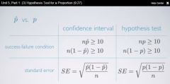
|
|
|
Week 06
T or F When comparing two means or proportions, one is working with two different groups but observing the same sample stastic among the groups to see how they differ? |

True. See question at left. where Coursera students are compared to US population on the general opinion of the separate groups on hand gun possession.
|
|
|
Week 06 |
It is
point estimate +- margin of error where the point estimate could be a mean or proportion and the margin of error takes different variables depending on the type of distribution. |
|
|
Week 06
What is a GOF Test, and what is it testing? |
It is a goodness of fit test, and it's testing how well the data fit the expected counts, for example, the goodness of fitness test with the chi-square GOF test.
|
|
|
Week 06
What are the segments of a single categorical variable called? |
Levels
|
|
|
Week 06
Conceptually, discuss the anatomy of a test statistic. |
|
|
|
Week 06
In general terms, discuss the chi-square statistic . Describe the greek letter used? |
when dealing with counts and investigating how far the observed counts are from the expected counts, we use a new test statistic called the chi-square (χ² ) statistic.
The greek letter is chi χ |
|
|
Week 06
When referring to cells in a χ contingency table, what is the word "cells" referring too? |
It is referring to the "levels" of the categorical variables.
|
|
|
Week 06
Why square with χ (chi)? |
|
|
|
Week 06
T or F A higher or lower, in the case where the test statistic is left of expected value, test statistic means a higher deviation from the null hypothesis? Why? |
T, because the test stastic represents the deviation from the expected value in terms of the expected value's STANDARD deviation.
|
|
|
Week 06
What is the function for the χ square test statistic in R? |

It is pchisq and the arguments in order are χ² test statistic, the degrees of freedom and the compliment of the lower tail as shown left.
|
|
|
Week 06
Describe the mechanics of the chi-square test of independpence for two categorical variables? |
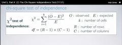
It is similar to the chi-square GOF test and is shown left. The difference is how the df are calculated. Remember for the GOF test it was simply df = k - 1
Remember, the null hypothesis says there is nothing going on (they're independent) while the alternative hypothesis states there is something going on (there is a dependence). |
|
|
Week 06
How does one calculate the expected values for a two way table? |
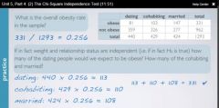
takes the rows, add them up, divide the result by the total as shown left. continue this process until all expected values are calculated.
|
|
|
What is the difference between a χ² GOF test and a χ² independence test?
|
The GOF test involves one categorical variable with more than 2 levels, and a independence test involves two categorical variables with at least one having more than 2 levels.
|
|
|
Week 07
T or F Linear regression assumes that the relationship between two variables, x and y, can be modeled by a straight line. Describe the equation for a straight line in terms of β coefficients |
For the regression case, the statistical model is as follows. Given a (random) sample the relation between the observations Yi and the independent variables Xij is formulated as
y = β0 + β1x |
|
|
Week 07
What is a coefficient? |
In mathematics, a coefficient is a multiplicative factor in some term of a polynomial, a series or any expression; it is usually a number, but in any case does not involve any variables.
7x^2 - 3xy + 1.5 + y For instance inthe first two terms respectively have the coefficients 7 and −3. The third term 1.5 is a constant. The final term does not have any explicitly written coefficient, but is considered to have coefficient 1, since multiplying by that factor would not change the term. Often coefficients are numbers as in this example, although they could be parameters of the problem, as a, b, and c, where "c" is a constant, in ax^2 + bx + c |
|
|
Week 07
When we use x to predict y, we usually call x the explanatory or _______________ variable, and we call y the response. |
predictor |
|
|
Week 07
Is correlation a statistic? |
Yes.
pg 316, Section 7.1 Line Fitting, Residuals, and Correlation |
|
|
Week 07
_____________ are the leftover variation in the data after accounting for the model fit. What is the equation? |
Residuals
Data = Fit + Residual |
|
|
Week 07
If an observation is above the regression line, then its residual, the vertical distance from the observation to the line, is ________________. Observations ____________ the line have negative residuals. |
positive, below.
|
|
|
Week 07
The size of a residual is usually discussed in terms of its ________________ value. |
absolute
|
|
|
Week 07
What is the equation for the residual difference? |
e(i) = y(i) - y-hat(i) where y(i) is the actual representation of the data and y-hat(i) is the point estimate based on the model.
|
|
|
Week 07
Residuals are ________________ in predicting how well a model fits a data set. |
helpful |
|
|
Week 07
Correlation, which always takes values between ____ and ___________, describes the __________ of the linear relationship between two ____________. We denote the correlation by R. |
-1, 1, strength, variables
|
|
|
Week 07
Interpret correlation of two variables as it relates to the computation of the correlation lying at or between -1 to 1 |
Only when the relationship is perfectly linear is the correlation either -1 or 1.
If the relationship is strong and positive, the correlation will be near +1. If it is strong and negative, it will be near -1. If there's no apparent linear relationship between two variables, then the correlation will be near zero. |
|
|
Week 07
The correlation is intended to ____________ the strength of a linear trend. |
indicate.
|
|
|
Week 07
Nonlinear trends, even when strong, sometimes produce correlations that do not reflect the strength of the ________________. |
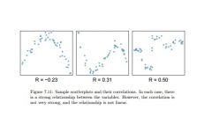
relationship
|
|
|
Week 07 What is the formula to compute the correlation for observations? |
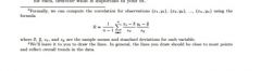
pg 322 OpenIntro Statistics |
|
|
Week 07 What is the method behind fitting a line by least squares regression? |
By choosing the line that minimizes the sum of the squared residuals |
|
|
Week 07 Least squares regression is a more _______________ approach to fitting a line as opposed to doing it "by eye" |
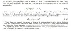
rigoruous |
|

Week 07 Give three possible reasons to choose Criterion 7.10 over 7.9 for fitting a line to a dataset. |
The first two reasons are largely for tradition and convenience; the last reason explains why Criterion 7.10 is typically most helpful |
|
|
Week 07 What are the conditions for the least squares line? |
When fitting a least squares line, we generally require
Note: Be cautious about applying regression to data collected sequentially in what is called a time series. |
|
|
Week 07 Be _______________ about applying regression to data collected sequentially in what is call a time ___________. Such data may have an _________________ structure that should be considered in a model and analysis. |
cautious, series underlying |
|
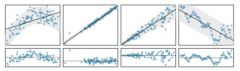
In the 4 paired panels left, apply and discuss the conditions for the least squares line. |
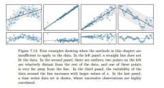
|
|
|
Week 07 Describe the correct code and output for all required testing techniques. |
- One numerical and one categorical variable (with only 2 levels): hypothesis test + confidence intervalparameter of interest = difference between two means (theoretical or simulation)parameter of interest = difference between two medians (simulation only)- One numerical and one categorical variable (with more than 2 levels): hypothesis test onlycompare means across several groupsno defined parameter of interest, ANOVA and pairwise tests (theoretical only)- Two categorical variables (each with only 2 levels): hypothesis test + confidence intervalparameter of interest = difference between two proportions (theoretical if success-failure condition met, simulation if not)- Two categorical variables (either one or both with more than 2 levels): hypothesis test onlycompare proportions across several groupsno defined parameter of interest, Chi-square test only (theoretical if expected sample size condition met, simulation if not) |
|
|
Week 07 In practice, this estimation is done using a computer in the same way that other estimates, like a sample mean, can be estiamted using a computer or calculator. However, we can also find the parameter estimates by applying two properties of the least squares line. What are they? |
|
|
|
Week 07 How does one interpret the parameters estimated by least squares? |
The slope diescribes the estimated difference in the y response bariable if the explanatory variable x for a case happened to be one unit larger. The y-intercept describes the average outcome of y if x = 0 and the linear model is valid all the way to x = 0, which in many applications is not the case. |
|
|
Week 07 Linear models can be used to __________________ the relationship between two variables. However, these models have ____________ limitations. Linear regression is simply a _________________ framework. The ______________ is almost always much more complex than our simple line. |
approximate, real, modeling, truth |
|
|
Week 07 Applying a model estimate to values outside the realm of the original data is called _____________________________. Generally, a linear model is only an approximation of the real relationship between _________ variables. If we extrapolate, we're making an unreliable _______ that the approximate linear relationship will be valid in places where it has not been analyzed. |
extrapolation, two, bet |
|
|
Week 07
What is R-squared (R^2)? |
Where correlation (R) describes the strength of a linear relationship, R-squared explains the strength of a linear fit, that is, how closely does the data cluster around the linear fit.
R^2 describes the amount of variation in the response variable that is explained by the least squares line. |
|
|
Week 07 Exercise 7.21, pg 330, If a linear model has a very strong negative relationship with a correlation of -0.97, how much of the variation in the response is explained by the explanatory variable? |
About R^2 = (-0.97)^2 of the variation is explained by the linear model. |
|
|
Week 07 For categorical predictors with just two levels, the linearity assumption will always be __________________. |
satisfied |
|
|
Week 07 Outliers in regression are _________________ that fall far from the "cloud" of points. These points are especially important because they can have a strong _____________ on the least squares line. |
observations, influence |
|
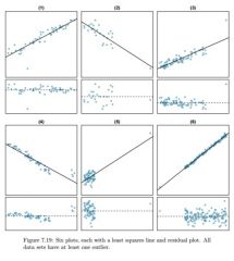
Week 06 In the 6 panels and the associated residual plot, explain the influence of the outlier on the linear regregression fit. |
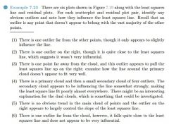
|
|
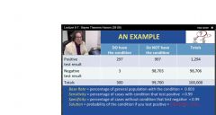
Week 03 When applying Bayes' Theorem (or two-way table) to the idea of a test such as with ____________________, that is, the probability you will test positive to some test (e.g. cancer, aids, drug tests, athletes included, eyewitnesses (given an accurate account), and standardized test (fail etc.) given you have the condition, the theorem allows us to determine the opposite, i.e., what is the probability you _____________ have the condition given you tested positive. Written as follows, we start with p(+|e) and end with p(e|+). Notice the _____________ to p-value as p-value is the probability of the expected or more outcome given the hypothesis, i.e. p(e|h) The opposite probability is called the _______________ probability. In general, one starts with _____________ probabilities, ________________ conditional probabilities, and ends with ____________ probabilities. Last, discuss the terminology associated with the two-way table left in terms of probabilities |
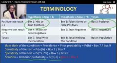
sensitivity, ACTUALLY similarity posterior marginal, determines, posterior |
|
|
Week 02 In terms of base rates, discuss a low base rate as it relates to a positive test. |
If you've a screening test with a low base rate or prevalence and you do not have any symptoms that put you in a special category, then you should get a second test before you jump to any conclusions. If you've a second test it puts you in a group with a higher prevalence or base rate, then the probability going to go up. Most doctors know this and that's why they order a second test but patients don't so they get worried. |
|
|
Week 02 Derive Bayes' Theorem |
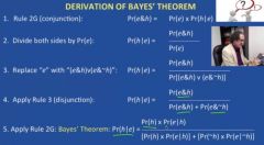
|
|
|
Week 07 Points that fall horizontally away from the center of "the cloud" tend to pull harder on the line, so we call them points with high ________________. These points can strongly influence the _________ of the least squares line and are called _________ points. Usually we can say a point is influential if, had we fitted the line withoutit, the influential point would have been unusually __________ from the least squares line. |
leverage, slope, influential far |
|
|
Week 07 It is __________ to remove outliers. __________ do this without a very good reason. |
tempting, DON'T |
|
|
Week 07 Be __________ about using a categorical predictor when one of the levels has very few observations. When this happens, those few observations become ______________ points. |
cautious, influential |
|
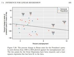
Week 07 Elections for members of the US House of REpresentatives occur every two years, coinciding every four years with US Presidential election. The set of House elections occurring during the middle of a Presidential term are called midterm elections. In America's two-party system, one political theory suggests the higher the unemployment rate, the worse the President's party will in the midter elections. To assess the validty of this claim, we can compkie historical data and look for a connection. We condinder every midterm election from 1898 to 2010, with the exception of those elections during the Great Depression. Figure 7.20 shows these data and the least-square line. The figure at left shows thes data and the least-squares regression line % change in House seats for President's party = -6.71 - 1.00 x (unemployment rate) We consider the % change in the number of seats of the President's party (e.g. percent change in the number of seats for Democrats in 2010) against the unemployment rate. Examining the data, there are no clear deviations from linearity, the constant variance condition, or in the normality of residuals (though we don't examine a normal probability plot here) While the data are collected sequentially, a separate analysis was used to check for any apparent correlation between successive observations; no such correclation was found. The data for the Great Depression (1934 and 1938) were removed becaouse the unemployment rate was 21% and 18%, respectively. Do you agree that they should be removed for this investigation? Why or why not? There's negative slope in the line. However, this slope ( and the y-intercept) are only estimates of the parameter values. We might wonder, is this convincing evidence that the "true" linear model has a negative slope? That is, do the provide strong evidence that the political theory is accurate? How would one state this investigation into a one-sided statistical hypothesis test: |
There are two considerations. Each of these points would have very high levrage on any least-squares regression line, and years with such high unemployment may not help us understand what would happen in other years where the unemployment is on modestly high. On the other hadn, these are exceptional cases, and we would be discarding important information if we exclude them from a final analysis. H(null): β1 = 0. The true linear model has a slope zero. H(alternative): β1 < 0. The true linear model has a slope less than zero. The higher the unemployment, the greater the loss for the President's party in the House of Representatives. To assess the hypotheses, we identify a standard error for the estimate, compute an appropriate test statistic, and identify the p-value |
|
|
Week 07 We usually rely on statistical _______________ to identify point estimates and standard errors for parameters of a regression line. |
software |
|
|
Week 07 Don't ________________ use the p-value from regression output |
carelessly The last column in regression output often lists p-values for one particular hypothesis: a two-sided test where the null value is zero. If your test is one-sided and the point estimate is in the direction of H(alternative), then you can halve the software's p-value to get the one-tail area. If neither of these scenarios match your hypothesis test, be cautious about using the software ouput to obtain the p-value. |
|
|
Week 07 R^2 describes the _______________ of variability in the response variable (y) explained by the explanatory variable (x). If this proportion is large, then this ____________ a linear relationship exists between the variables. If this proportion is small, then the evidence provided by the data may not be convincing. Why is the condition important? |
proportion The condition is important as it offers an alternative to the test statistic in determining the strength of evidence for a relationship between the explanatory and response variables. This concept--considering the amount of variability in the response variable explained by the exlanatory variable--is a key component in some statistical techniques. The analysis of variance (ANOVA) technique uses this general principle. The method states that if enough variability is explained away by the categories, then we conclude the mean varied between the categories. On the other hand, we MIGHT NOT be convicne if only a little variability is explained. ANOVA can be further employed in advanced regression modeling to evaluate the inlusion of explanatory variables, though these details are left to a later course. |
|
|
Week 07 What is the function to calculate correlation in R? Describes it arguments. |
the function is cor(input1, input2) input1 and input2 are the variables that one seeks to correlate. They're vectors. |
|
|
Week 07 Describe the following function and its output.
|
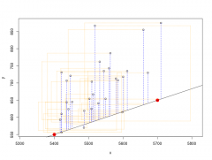
This function will first draw a scatterplot of the first two arguments x and y. Then it draws two points (x1, y1) and (x2, y2) that are shown as red circles. These points are used to draw the line that represents the regression estimate. The line you specified is shown in black and the residuals in blue. Note that there are 30 residuals, one for each of the 30 observations. Recall that the residuals are the difference between the observed values and the values predicted by the line:ei=yi−yi^The most common way to do linear regression is to select the line that minimizes the sum of squared residuals. To visualize the squared residuals, you can rerun the plot_ss() command and add the argument showSquares = TRUE.plot_ss(x = mlb11$at_bats, y = mlb11$runs, x1, y1, x2, y2, showSquares = TRUE)Note that the output from the plot_ss() function provides you with the slope and intercept of your line as well as the sum of squares. |
|
|
Week 08 What is logistic regression? |
It is applying regression to categorical variables whereby one predicts categorical outcomes with two categories.
|
|
|
Week 08 While we remain cautious about making any ______________ interpretations using multiple regression, such models are a common first step in providing evidence of a causal connection. |
causal |
|
|
Week 08 Just as with the single predictor, a multiple regression ____________ may be missing important components or it might not precisely represent the relationship between the outcome and the available explanatory variables. |
model |
|
|
Week 08 How are the coefficients of a multiple regression fit estimated? |
They are selected in the same that they were for a single predictior, that is, select coefficients that minimize the sum of the squared residuals. |
|
|
Week 08 A multiple regression model is a _______________ model with many predictors. |
linear
|
|
|
Week 08 What is the equation for R^2 with multiple regression? |
R^2 = 1 - (variability in residuals/variablility in the outcome) = 1 - (Var(e(i))/Var(y(i))) |
|
|
Week 08 What is adjusted R^2? |
Adjusted R^2 for multiple regression is R^2(adj) = 1 - (Var(e(i))/(n-k-1)/Var(y(i)) /(n-1)) = 1 - Var(e(i)) / Var(y(i)) x n-1 / (n-k-1) where n is the number of cases used to fit the model and k is the number of predictor variables in the model |
|
|
Week 08 Will R^2(adj) be smaller or larger than R^2 unadjusted? Why or why not? |
Because k is never negative, the adjusted R^2 will be smaller - often times just a little smaller - than the undajusted r^2. The reasoning behind the adjusted R^2 lies in the degrees of freedom associated with each variance. |
|
|
Week 08 The best model is ___________ always the most complicated. |
not |
|
|
Week 08 Sometimes including ______________ that are not evidently important can actually reduce the accuracy of predictions in multiple regression. |
variables |
|
|
Week 08 In multiple regression, the model that includes all available explanatory variables is often referred to as a ______________ model. |
full |
|
|
Week 08 What is an interaction variable? |
This is an advanced statistical concept when modeling, using correlation, interaction variables are used to adjust for categorical variables that have a domain, for example, of 0 or 1, that allows the model to shift (be displaced) to compensate for the opposing levels of the variable. In other words, one could have two parallel lines say for smokers and non-smokers where the variable adds or substracts from the model. Typically, these lines might be parallel but if they are not the interaction variable compensates for that. |
|
|
Week 08 What is the equation for R^2 in using ANOVA outputs? |

R^2 = explained variability/total variability. See the image, left. |
|
|
How would one use the anova function from R to create an anova table using a variable that was assigned to a lm function (linear model) function? |

See image, left. |
|
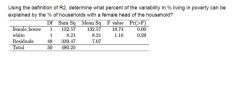
Week 08 Solve the problem, left. |
132.57 / 480.25 = 27.6% Note that the variability attributable only to female head of household is used. |
|
|
Week 08 What happens to R ^ 2 when a new variable is added to the model? |
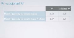
It increases because the explained variability increases the denominator at a faster rate than the total variability increases. However, if the additional variable does not add any information or is not related the R^2 decreases. |
|
|
Week 08 List the properties of adjusted R^2. |
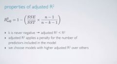
|
|
|
Week 08 T or F Adjusted R^2 tells us the percentage of variability in the response variable explained by the model. |
False. This is the defintion of R^2. adjusted R^2 not only gives the percentage of the response variable explained by the model, it also has a penalty for the number of predictors included in the model. |
|
|
Week 08 What is multicollinearity? |
It is the inclusion of collinear predictors in a model. |
|
|
Week 08 Predictors are also called _______________ variables, so they should be independent of each other. They should __________ be collinear. |
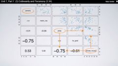
independent, not Notice how white and female_house are highly correlated. Therefore, they are dependent on each other so the variable white should not be added to the model as it brings nothing new to the table. |
|
|
Week 08 How does multicollinearity affect a model? |
It COMPLICATES model estimation. |
|
|
Week 08 What is parsimony? |
|
|
|
Week 08 What is Occam's razor? |
The idea of parsimony stems from this concept and states that among competing hypotheses, the one with the fewest assumptions should be selected.
|
|
|
Week 08 Addition of collinear variables can result in ____________ estimates of the regression parameters. |
biased |
|
|
Week 08 While it's impossible to avoid collinearity from arising in observational data, __________ are usually designed to control for correlated predictors. |
experiments |
|
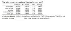
Week 08 How would one setup a hypothesis test for the ouput, left? |
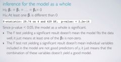
Null, there's nothing going on with the slopes or they're all zero. Alternative, there's at least one slope that is different from zero. |
|
|
Week 08 Explain how the calculation of degrees of freedom for a single predictor (n-2) is consistent with the calculation for multiple predictors? (n-k-1)? What does the one represent in the formula n-k-1? |
With a single predictor k or the number of predictors is 1, therefore (n-k-1) is equal to n-1-1 which is equal to n-2. It represents the intercept since a degree of freedom is lost for it. |
|
|
Model selection is a science and an __________. Variables can be chosen on expert __________. |
art, opinion. |
|
|
Week 08 What is the criteria for model selection? |
|
|
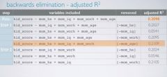
Week 08 Discuss the image at left using the backwards elimination model selection and adjusted R^2. |
Discuss the steps. Notice how variables are removed to determine if a higher adjusted R^2 is arrived at that previously noticed. Continue this process, searching for a higher adjusted R^2. |
|

Week 08 Discuss the image at left using the backwards elimination model and p-value. |
Start with the variable having the highest p-value that is not statistically significant. Re-run the model and repeat process until all variables are significant. |
|
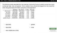
Week 08 Looking at the image at left using backward model selection and p-value which variable should be removed first? |
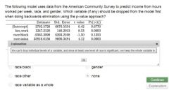
None. This is a trick question but no variable should be removed even though race:black does not have statistical significance since it is a level (category) of the race variable and at least one of those levels, asian, has statistical significance. In order to drop a categorical variable, none of the levels can have statisical significance. |
|
|
Week 08 Contrast using adjusted R^2 to p-value approach criterion in selecting a model. |
|
|
|
Week 08 Variables can be included in (or __________________ from) the model based on expert opinion. For example, if you're studying a certain variable, you might choose to leave it in the model regardless of whether it's significant or yield a __________ adjusted R^2 |
eliminated, higher |
|
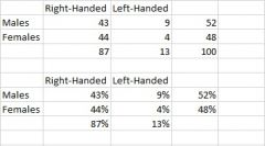
What is a contingency table? What forms can it take? The table at left that shows count data; explain how it would be explained in percentages (probabilities)? For the graph left, explain how the count data and probabilities below would change if the count data were doubled for each cell. |
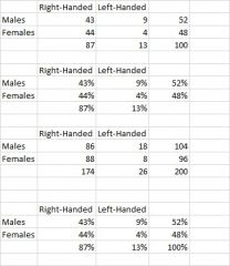
When analysis of categorical data is concerned with more than one variable, two-way tables (also known as contingency tables are employed. (Source: http://www.stat.yale.edu/Courses/1997-98/101/chisq.htm) In statistics, a contingency table (also referred to as cross tabulation or crosstab) is a type of table in a matrix format that displays the (multivariate) frequency distribution of the variables. They are heavily used in survey research, business intelligence, engineering and scientific research. They provide a basic picture of the interrelation between two variables and can help find interactions between them. The term contingency table was first used by Karl Pearson in "On the Theory of Contingency and Its Relation to Association and Normal Correlation",[1] part of the Drapers' Company Research Memoirs Biometric Series I published in 1904. The count data would change as shown in table 3. However, the probabilities would remain the same. |
|

Explain how the graph at left is a contingency table. What is different about this contingency table? How does the conjoined information center match the original results? |
It is a two-way contingency table categories of B and b. It is different in that the marginal data is at the top and left instead of right and bottom which is the normal format. Originally, observing the marginal data, there's 120 Bs and 80 bs. Adding up the center data one gets 120 Bs by 36*2+24+24 = 120 and 80 bs by 24*2+ 16*2 = 80 This graph is designed to show if 60% of the male population has a Brown eye allele (gene variation) and 40% has a blue eye allele and 60% of the female population has a Brown eye allele and 40% has a blue eye allele then the results (center) keeps the same proportion if they are conjoined as in the graph. |
|
|
Lecture 06 Probability Is in Our Genes |
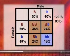
These theorem says that if a population has certain characteristics in a given proportion then if the population is randomly combined then the resulting population will have the same proportions. This is indicated in the graph at left with Brown and blue alleles (gene variations). It is counter-intuitive but over time it seems that if there's a recessive gene containing a blue allele, one would think it would be washed over time but according to this theory, it will remain in the same proportion. This applies to rare diseases like cystic fibrosis. That is, over time scientist expect the percentage of people with the disease will remain the same over time. Of course it will die if there's a smaller chance of reproduction. |
|
|
Week 02 Describe the difference between disjunction (or) and conjuction (and) mathematical |
A conjunction multiplies independent ( or dependent in the case of conditional probabilities ) events to yield a probability. In the case of mutually exclusive events, the probability is zero. A disjunction (or) adds probabilities to arrive at the overall probability of separate events. Conjunction and disjunctions can be combined to arrive at probabilities. One sees this with distributions such as binomial distrubutions, frequently. |
|
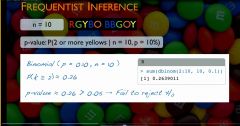
Week 02 Last video of week 02 discussed frequentist vs. ____________. Describe how the following code in R (sum(dbinom(2:10, 10, 0.1)) would be calculated in Excel. |
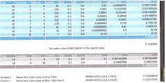
This code describes the probability of at least 2 yellow M&Ms being pulled ( a success ). There are ways this could be calculated using excel: 1. List 8 rows as shown in table 1 then sum 2. List 2 rows as shown in table 2 sum then take compliment 3. Use binom.dist function with TRUE argument to calculate 2. above and take complement. |
|
|
|
|
|
|
What is the relationship between a hypothesis, conjecture and proposition? |
A hypothesis is a testable conjecture. A conjecture is an unproven proposition. |
|
|
We make observations where we can find relationships to _______________ outcomes. If we can find casual relationships, then we might be able to produce, ___________ or eliminate the results. |
predict, reduce |