Reading...
![]()
Play button
![]()
Play button
![]()
Use LEFT and RIGHT arrow keys to navigate between flashcards;
Use UP and DOWN arrow keys to flip the card;
H to show hint;
A reads text to speech;
11 Cards in this Set
- Front
- Back
|
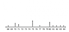
The heights of 20 basketball players, in inches, are given. Create a dot plot to show the data. 68, 70, 70, 71, 75, 80, 81, 82, 84, 75, 75, 80, 75, 77, 75, 80, 83, 80, 71, 70
|
|
|
|
The number of chocolate candies per bag of trail mix is given. Create a histogram to show the data. 50, 42, 99, 45, 68, 32, 67, 91, 61, 31, 75, 39, 62, 64, 49, 55, 51, 33, 97, 96, 64, 82
|
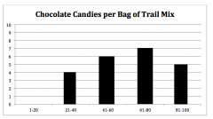
(The intervals may vary, but your histogram should look similar to this one.)
|
|
|
Draw a box plot to represent the following data: 3, 6, 8, 10, 4, 8, 9, 15, 4, 8, 10
|
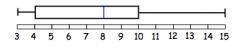
Q1: 4 Q2: 8 Q3: 10
|
|
|
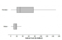
75 female and 24 male college students reported the cost (in dollars) of his or her most recent haircut. The data are summaried in the table. Using the minimum, maximum, quartiles, and median, sketch two side by side box plots to compare the hair cut costs between males and females in this student's school.
|
|
|
|
75 female and 24 male college students reported the cost (in dollars) of his or her most recent haircut. The data are summaried in the table. How would you describe the difference in haircut costs between males and females? Be sure you discuss differences/ similarities in shape, center, and spread.
|
Both boxplots show distributions that are skewed to the right. It makes sense that most haircuts will not cost too much, but a few students will spend a large amount. Since the cost will always be a positive number, the minimum cannot be less than 0 and there is a long right tail. The centers and spreads are quite different. The median cost for females is about twice that of males, and there is much more variability in the costs for women. The IQR for women is %55, while for men it is $10.75.
|
|
|
75 female and 24 male college students reported the cost (in dollars) of his or her most recent haircut. The data are summaried in the table. Why is the mean greater than the median for both males and females? Explain your reasoning.
|
We should not be suprised that the mean is larger than the median because the distribution appears to be skewed to the right. The mean averages all the values in the data, so is "pulled" toward the high values. The median is the 50th percentile and is resistant to the extreme values.
|
|
|
75 female and 24 male college students reported the cost (in dollars) of his or her most recent haircut. The data are summaried in the table. Is the median or mean a more appropriate choice for describing the "centers" of these two distributions?
|
Since the median gives a better description of the center, or a "typical" haircut cost, it is more appropriate. The mean doesn't give us a good idea of what we could expect for a typical student's haircut cost. It is best to only use the mean when the data distribution is reasonably symmetric.
|
|
|
Suppose that SAT math scores for a particular year are approximately normall distributed with a mean of 510 and a standard deviation of 100. What is the probability that a randomly selected score is greater than 610?
|
The score 610 is one standard deviation greater than the mean, so the tail area above that is about half of 0.32 or 0.16.
|
|
|
Suppose that SAT math scores for a particular year are approximately normall distributed with a mean of 510 and a standard deviation of 100. What is the probability that a randomly selected score is greater than 710?
|
The score 710 is two standard deviations above the mean, so the tail area above that is about half of 0.05 or 0.025.
|
|
|
Suppose that SAT math scores for a particular year are approximately normall distributed with a mean of 510 and a standard deviation of 100. What is the probability that a randomly selected score is between 410 and 710?
|
The area under a normal curve from one standard deviation below the mean to two standard deviations above the mean is about 0.815.
|
|
|
Suppose that SAT math scores for a particular year are approximately normall distributed with a mean of 510 and a standard deviation of 100. If a student is known to score 750, what is the student's percentile score? (A percentile score is the proportion of scores below the score in question)
|
The percentile score is 99.18%. This can be found by calculating the z-score, which is 2.4
|