Statistics, Ch. 1 (Intro)

Front 1

The degree to which a statistical model represents the data collected

Back 1

The fit of the model

Front 2

A hypothetical value that can be calculated for any data set (not necessarily actually observed in the data set)

Back 2

The mean value

Front 3

The deviance between the observed data and the model

Back 3

The error in the model

(the bigger the number, the poorer the fit of the model)

Front 4

Calculate the magnitude of deviance

Back 4

Subtract the mean value from each of the observed values.

(For example, in a problem where the mean amount of friends for a lecturer is 2.6. And lecturer 1 had only 1 friend, so the difference is x1 - x = 1 - 2.6 = - 1.6. Our model OVERESTIMATES his popularity, it predicts he will have 2.6 friends but he only has 1)

Front 5

A good measure of how well the mean represents the data (how well our model fits the data)

Back 5

Sum of squared error

Front 6

Variance

Back 6

Sum of squared error (SS) / sample size minus 1 (n - 1)

Front 7

Standard deviation

Back 7

Variance gives an answer in united squared (because each error was squared in the calculation)

SO, the square root of the variance is needed. This is called the Standard Deviation - a measure of how well the mean represents the data.

Front 8

Standard deviation: Size

Back 8

Small standard deviations (relative to the value of the mean itself) indicate that data points are close to the mean

A large standard deviation (relative to the mean) indicates that the data points are distant from the mean

Front 9

If we're looking at how well a model fits the data, then we generallly look at deviation from the model, we look at the sum of squared error

Back 9

deviation = sum (observed - model)2

Front 10

A graph of how many times each score occurs

(A graph plotting values of observations on the horizontal axis, with a bar showing how many times each value ocurred in the data set)

Back 10

Frequency Distribution / Histogram

Front 11

The score that occurs most frequently in the data set

Back 11

The mode

Front 12

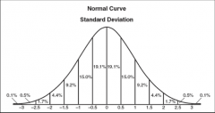
The normal distribution

Back 12

Front 13

Frequency Distribution: Symmetry

Back 13

Skewness.

Positively skewed - the frequent scores are clustered at the lower end and the tail points towards the higher / more positive scores

Negatively skewed - the frequent scores are clustered at the higher end of and the tail points towards the lower, more negative scores

Front 14

Frequency Distribution: Pointyness

Back 14

Kurtosis: the degree to which scores cluster in the tails of the distribution.

Platykurtic - many scores in the tails, and is therefore flat

Leptokurtic - thin in the tails, so look quite pointy

Front 15

Standard Deviation & Shape of Distribution

Back 15

As the standard deviation gets larger, the distribution gets wider

Front 16

Probability distributions

Back 16

Statisticians have identified several common distributions. For each one, they have worked out mathematical formulae that specify idealised versions of these distributions, called Probability Distributions. From one of these distributions, it is possible to calculate the probability of getting particular scores based on the frequencies with which a particular score occurs in a distribution with these common shapes.

Front 17

Z Scores

Back 17

Any data set (even if it has a mean of 567 and an SD of 52.98!) can be converted into a data set that has a mean of 0 and a standard deviation of 1

Front 18

Z Scores: Equation

Back 18

First, to centre the data at zero, we take each score and subtract it from the mean of all scores. Then, we divide the resulting score by the standard deviation to ensure all data have a standard deviation of 1

z = score - (mean of scores) / SD

Front 19

95% of z scores lie between

Back 19

- 1.96 and 1.96

Front 20

99% of z scores lie between

Back 20

- 2.58 and 2.58

Front 21

99.9% of z scores lie between

Back 21

- 3.29 and 3.29

Front 22

How well a particular sample represents the population

Back 22

Standard Error