Stats Ii Midterm (2Nd Half Of Content)

Front 1

are quadratic functions only useful for approximating the shape of an upward or downward facing curve?

Back 1

No, they can approximate many different shapes (there doesn't necessarily need to be a minimum and maximum in the actual data)

Front 2

Why should you try adding a quadratic (x^2) term to your regression model?

Back 2

good way to gauge the presence of nonlinearity because quadratic functions can approximate many different shapes...BUT, just because the quadratic fits better than the linear doesn't mean there's an actual reversal of direction, especially if the maximum or minimum is outside the range of the data

Front 3

what does the Stata command "quietly adjust indvar1 indvar2 indvar3 indvar4, gen(predicted) and then "line predicted indvar5, sort" do?

Back 3

The first command generates the predicted values of the dependent variable when the independent variables listed within the command are set at their means (note: make sure you leave out the independent variable whose relationship with y you're interested in looking at). The second command draws a line using the predicted values of the dependent variable and the independent variable of interest. This allows you to get a better idea of what shape the relationship between the dependent variable and the independent variable of interest takes on

Front 4

what are some of the most widely used transformations of variables?

Back 4

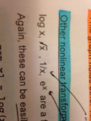
log(x), square root of x, 1/x (reciprocal of x), and e^x (exponential function of x)

Front 5

which variables should you transform when testing for nonlinearity of the relationship between the dependent and independent variables?

Back 5

you should avoid transformations of the dependent variable at all costs, UNLESS taking the log of the dependent variable

Front 6

how can you implement these transformations in Stata?

Back 6

a) gen x1 = log(x)
b) gen x2 = sqrt(x)
c) gen x3 = 1/x
d) gen x4 = exp(x)

Front 7

what is a warning to keep in mind when working with these transformations and most other transformations?

Back 7

all four of these transformations (logarithms, recriprocals, exponentials) require a measurement of x at the ratio level. The shape of the curve DEPENDS on the 0 point of the x variable, so you CAN'T have an arbitrary zero point. This warning does NOT apply, however, to the quadratic (x^2) or higher-order polynomials (e.g. x^3??)

Front 8

what do these 4 common transformations look like when graphed? (i.e. what kind of nonlinear relationships between the dependent and independent variable do they represent?)

Back 8

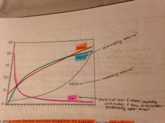
log(x) = "diminishing returns" (dependent variable increases at a high rate in beginning, but then continues to increase but at a lower and lower rate overtime)...exp(x) = "increasing returns" (dependent variable increases at a low rate in the beginning, but then increases at a higher and higher rate overtime)...1/x: dependent variable starts out at a very high value and then rapidly diminishes and then at some point begins to diminish more slowly/gradually)

Front 9

what is the difference between sqrt(x) function and log(x) function?

Back 9

they have a similar shape, in that the independent variable cannot go below 0 (line is always to right of vertical axis). The difference is that in a sqrt(x) function, the y variable also cannot take a value below 0; in the log(x) function, the y variable can take values below 0, and in fact y will approach negative infinity as x gets closer and closer to 0

Front 10

what are the two types of nonlinearity for multiple regression?

Back 10

1. Nonlinearity in the variables: this is the kind we've been looking at so far. The general form is: y = b0 + b1f1(x1) + b2f2(x2) +...+bkfk(xk) + E, where "f1" means "some function" that we are applying to x1...could be sq. rt, log, exponent...In these cases, the functions can be any tranformations of the x's...this kind of nonlinearity can be easily handled by OLS regression simply by transforming the variables.
2. Nonlinearity in the parameters: The nonlinearity is some function applied to the parameters. Such models can usually be estimated by nonlinear least squares. That is, we still choose the coefficients to minimize the sum of square residuals. BUT the calculations are considerably more complex (usually iterative, meaning they involve successive approximations) and can often run into difficulties. The "nl" command in Stata can perform nonlinear least squares

Front 11

if a variable does not have a statistically significant effect on y in a linear regression model, should you test to see if it has a statistically sig. effect on y in a model that includes a nonlinear transformation of the variable in question?

Back 11

No. If it isn't significant in the original form, probably won't become significant after a transformation

Front 12

in what case can you transform models that are nonlinear in the parameters into linear models?

Back 12

By using logarithms (only works in some cases, however). For example, if have y = bo(x1^b1)*(x2^b2)*E, you can take the logarithm of both sides to get: log(y) = log(b0) + b1(log[x1]) + b2(log[x2]) + log(E). In this case, the coefficients in this model are called "elasticities" because they can be interpreted as closely approximating the percent change in y for a 1 percent increase in x

Front 13

when should you use a log transformation?

Back 13

when there is theoretical reason to believe that the relationship between the independent variable and the dependent variable is not linear. What's more, a log transformation will create a relationship in which there are diminishing returns to increases in the x variable...so need reason to believe that as x increases, its effect on y will slowly diminish.

Front 14

what are some empirical reasons for using a log transformation?

Back 14

using the log transformation will mitigate the problem of heteroskedasticity. This is because taking the log will make the distribution of the RESIDUALS more Normal, and if the distribution of the residuals is more Normal, this mitigates the problem of heteroskedasticity. Thus, it may be especially appealing to use log transformation when the distribution of the independent variable(s) or dependent variable is positively skewed (ie right-skewed). That being said, the primary reason for using log transformation should be theoretical.

Front 15

can you compare the adjusted R-squareds of a regression model with and without a log transformation?

Back 15

If you have performed a log transformation of the dependent variable, you CANNOT compare R-squared of this model w/ that of regression model without log transformation. However, if you have performed a log transformation of the INdependent variable, you CAN compare R-squared of this model w/ that of regression model without log transformation

Front 16

what are some cautions about using log transformations?

Back 16

1. the variables should be measured at ratio level (with a natural, rather than arbitrary, 0)
2. There cannot be any zero or negative observations of the variable that will undergo the log transformation
3. Log transformations will fundamentally alter the relationship between IV and DV, which may or may not be conceptually desirable...i.e. you need to make sure that this change in the relationship makes sense

Front 17

what can you do if there are zero or negative observations but you want to use the log transformation?

Back 17

you can add a constant (generally 0.5) to each observation. You do this by taking log(x+k) e.g. log(x+0.5)

Front 18

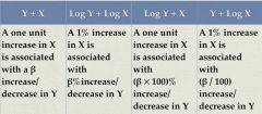
what is the interpretation of the coefficient on the independent variable for a regression model where the dependent variable is y and independent variable is x?

Back 18

a one unit increase in x is associated with a b increase/decrease in y

Front 19

what is the interpretation of the coefficient on the independent variable for a regression model where the dependent variable is log(y) and independent variable is log(x)?

Back 19

A 1% increase in x is associated with a b% increase/decrease in y

Front 20

what is the interpretation of the coefficient on the independent variable for a regression model where the dependent variable is log(y) and independent variable is x?

Back 20

a one unit increase in x is associated with a b*100% increase/decrease in y (note: if the coefficient doesn't fall between -0.1 and +0.1, you should use the formula 100*(e^b) - 1...ie, a one unit increase in x is associated with a 100*(e^b) -1 increase/decrease in y

Front 21

what is the interpretation of the coefficient on the independent variable for a regression model where the dependent variable is y and independent variable is log(x)?

Back 21

a 1% increase in x is associated with a b/100 unit increase/decrease in y

Front 22

here's the chart in case it helps

Back 22

attached

Front 23

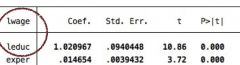
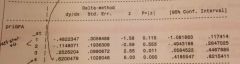
how would you interpret the coefficients on "leduc" and "exper" in this example?

Back 23

a 1% increase in education is associated with a 1.02% increase in wage.

a 1-unit increase in experience is associated with a 1.4% increase in wage

Front 24

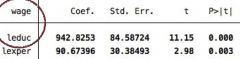
how would you interpret the coefficients on 'leduc' and 'lexper' in this example?

Back 24

a 1% increase in education is a associated with a 9.42 unit increase in wage

a 1% increase in experience is associated with a 0.9 unit increase in wage

Front 25

what are elasticities?

Back 25

when there is a log transformation on both the independent and dependent variables, i.e. log(x) and log(y). This will tell you what % change in y is associated with a 1% increase in x

Front 26

if the regression model is transformed from
y = exp(b0 + b1x1 + b2x2 +...+ bkxk + E) to
log(y) = b0 + b1x1 + b2x2 +...+bkxk + E, how do you interpret the regression coefficients (e.g. b1, b2, bk)? What is a common use of this transformation?

Back 26

100*[(e^b)-1] is the percent change in y for a one-unit increase in x
This transformation is commonly used when the dependent variable cannot be less than zero (like income)

Front 27

theoretically, what does the following model suggest about the relationship between x and y?
y = b0 + b1log(x) + E

Back 27

assuming that b1 is positive, this says that an increase in x produces increases in y, but that there are "diminishing returns" (i.e. a change in x from 1 to 2 will have a bigger effect than a change from 10 to 11). b1 can be interpreted as meaning that a 1% increase in x is associated with a b1/100 unit increase in y

Front 28

what is interaction?

Back 28

another type of nonlinearity. This is when the effect of x1 on y is NOT the same for every individual in the sample. Rather, the effect of x1 on y is affected by another independent variable (say, x2).

Front 29

what are 2 examples of an interaction?

Back 29

when the gender of individuals affects the effect of experience on wage. For example, the effect of experience on wage might be higher for women than for men, or vice versa

when the high school GPA of an individual affects the effect of SAT score on scholarship amount. For example, the effect of SAT score on scholarship amount may be greater for individuals with a lower GPA than for individuals with a higher GPA

Front 30

how do you express interaction within a regression model? For example, if the model without interaction looks like this:
y = b0 + b1x1 + b2x2 + E and you have reason to suspect that there is an interaction between x1 and x2

Back 30

y = b0 + b1x1 + b2x2 + b3x2x1 + E

"b1" = main effect of x1
"b2" = main effect of x2
"b3" = interaction term (interaction b/w x1 and x2)

Front 31

why do you need to include the "main effects" in the regression model for an interaction?

Back 31

because you want to test the significance of the interaction (does it really matter, or do the main effects account for all of the variation in y?)

Front 32

how do you interpret the main effects in a regression model that includes an interaction term?

Back 32

in the above example, the main effects are b1 and b2. b1 = the main effect of x1, when x2 = 0;
b2 = the main effect of x2, when x1 = 0

Front 33

if you include an interaction term in a regression model, do you interpret it as x1 influencing the effect of x2 on y or as x2 influencing the effect of x1 on y?

Back 33

interaction via a product term is symmetrical. This means that just as the effect of x1 depends on the level of x2, so also the effect of x2 depends on the level of x1. There are always two different ways to look at an interaction

Front 34

how should you interpret the standardized coefficients for the two variables in the interaction?

Back 34

you shouldn't; looking at the standardized coefficients for these 2 variables is useless in this situation

Front 35

what is the only situation in which you would NOT include the main effects in a regression model with an interaction term?

Back 35

when both variables are measured on a ratio scale and you have a strong theory. Otherwise, if you leave out the main effects, the model says that the effect of one variable is 0 when the other variable is 0

Front 36

is a product term (i.e b3x1x2) the only way to represent an interaction in a regression model?

Back 36

No, there are many other ways to represent interaction, e.g. x1/x2, but most of these require that at least one of the variables is measured on a ratio scale

Front 37

how do you interpret the results of an interaction?

Back 37

first, check if the p-value on the interaction coefficient is statistically significant and that the coefficient on the interaction term is not 0. Then, select a set of values for one of the two variables, say x1, and then calculate the effect of x2 on y for each of the different values of x1

Front 38

what's the relationship between interaction b/w x1 and x2 and correlation b/w x1 and x2?

Back 38

Nothing!! This is a common misunderstanding. Interaction is about how the effect of 1 variable depends on the value of another variable. It says NOTHING about the correlation between these 2 independent variables

Front 39

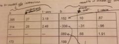
How would you interpret this chart?

Back 39

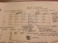
the first row, second b is the main effect of x1 (i.e. when x2 is set to equal 0, the effect of x1 on y)...the second row, second b is the main effect of x2 (i.e. when x1 is set to equal 0, the effect of x2 on y). The third row, second b is the interaction coefficient. The standardized coefficients after adding the interaction term don't tell us anything (b/c added an interaction term).

Front 40

how do you hand calculate the effect of x1 on y for different levels of x2? Please calculate as pertains to the chart on the previous flash card

Back 40

You multiply the value of x2 by the interaction coefficient and add this number to the main effect of x1, i.e. coefficient on x1 + interaction coefficient(value of x2)
0 (0.152 + 0.089*0) = 0.152
1 (0.152 + 0.089*1) = 0.241
2 (0.152 + 0.089*2) = 0.330
3 (0.152 + 0.089*3) = 0.419

Front 41

what is the interpretation of the hand calculations? What do they tell us about how x2 affects the effect of x1 on y?

Back 41

Interpretation: for an individual with a value of 3 for the variable x2, a one-unit increase in x1 is associated with a 0.419 unit increase in y. Our calculations also tell us that the effect of x1 on y is greater at higher values of x2

Front 42

how do you hand calculate the effect of x2 on y for different levels of x1? Please calculate

Back 42

You multiply the value of x1 by the interaction coefficient and add this number to the main effect of x2, i.e. coefficient on x2 + interaction coefficient(value of x1)
0 (-0.336 + 0.089*0) = -0.336
1 (-0.336 + 0.089*1) = -0.247
4 (-0.336 + 0.089*4) = 0.020
8 (0.152 + 0.089*8) = 0.376

Front 43

what is the interpretation of the hand calculations? What do they tell us about how x1 affects the effect of x2 on y?

Back 43

Interpretation: for an individual with a value of 4 for the variable x1, a one-unit increase in x2 is associated with a 0.020 unit increase in y. Our calculations also tell us that the effect of x2 on y is negative up until a certain point, after which it becomes positive and increases in degree as value of x1 increases

Front 44

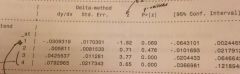
how do you interpret the attached stata output?

Back 44

here we are looking at how the independent variable priorGPA affects the effect of the other independent (attend) on the dependent variable (test score). We see that for people whose GPA is "1", a one unit increase in attendance is associated with a 0.030 decrease in test score. This seems very weird. As it turns out, the p-values for coefficient on attendance for individuals with GPAs of 1 and 2 are high, meaning that the effect of attendance on test score is not statistically significant for students who have GPAs of 1 or 2. For students w/ GPAs of 2, a one unit increase in attendance is associated with a 0.0058 unit increase in test score. For students w/ GPA of 3, a one unit increase in attendance is associated with a 0.042 increase in test score. The chart indicates that the positive effect of attendance on test score is higher for students with GPA of 4 than those w/ GPA of 3 and is not statistically significant for students with GPAs of 1 or 2.

Front 45

how do you interpret this table? x1 = priGPA, x2 = attendance, y = test score

Back 45

this shows us the effect of prior GPA on test score for people with different levels of attendance. Looking at the p-values, we see that prior GPA only has a statistically sig effect on test score when attendance rate is at level of 3 or 4. For people w/ a level 3 attendance rate, a one unit increase in prior GPA is associated with a 0.253 unit increase in test score. For people w/ a level 4 attendance rate, a one unit increase in prior GPA is associated with 0.62 unit increase in test score. In other words, prior GPA has a larger effect on test score for people with higher attendance rates

Front 46

what are dummy variables?

Back 46

They are used to represent dichotomous nominal variables. A dummy variable has only two possible values, 0 and 1. Using dummy variables makes it possible to use nominal variables as predictors. The choice of what category of a dichotomous nominal variable is represented by a value of "0" vs "1" is purely arbitrary, but you need to remember the choice in order to interpret the results properly

Front 47

do you use dummy variables as dependent or independent variables in a regression model?

Back 47

Either, though usually they work better as independent variables

Front 48

if y = hours of housework per week
x1 = sex (1 = female and 0 = male)
and you're calculating that = b0 + b1x1
then what does b0 =? what does b1=?
what kind of relationship are we using the regression model to explain?

Back 48

b0 = the mean of y for males
b1 = the difference between the mean of y for females and the mean of y for males (ybarF - ybarM), where the number being subtracted is the mean of y for the category that has a value of 0
we are using the regression model to explore whether or not gender effects the hours of housework an individual performs per week. If the mean hours of housework for men and women is equal, this means that there is no effect of x1 on y

Front 49

what is the t-test for b1 = 0 in the regression model with the dummy variable from the previous card?

Back 49

the t-test for b1 = 0 is exactly equivalent to the usual t-test for a difference b/w two means:
ybarF - ybarM/(pooled estimate of the standard deviation in the two groups*sqrt[1/n1 + 1/n2])
the difference in the mean of the two groups divided by the pooled estimate of the standard deviation in the two groups times sqrt of (1/the sample size of females + 1/the sample size of males)
note: the pooled standard deviation is the standard deviation of y, which we estimate by using the standard deviation of y in the sample

Front 50

why do we use a pooled estimate of the standard deviation in the two groups for a t-test for b1=0 in a regression model where the independent variable is a dummy variable?

Back 50

because this corresponds to the homoskedasticity assumption

Front 51

what happens if we add another independent variable to the regression model so that
y = hours of housework per week
x1 = gender (1=female, 0=male)
x2 = hours employed per week
we get yhat = b0 + b1x1 + b2x2
what does b0=?
what does b1=?
what does b2=?
what relationship are we trying to describe with this regression model?

Back 51

b0 = predicted hours of housework for unemployed males (i.e. x1 and x2 both set to 0)
b1 = difference in average housework hours of males and females, controlling for employed hours (adjusted difference in means)
b2 = effect of employed hours on housework hours, controlling for sex
we are seeing how gender affects the number of hours of housework an individual performs per week, holding number of hours employed per week constant

Front 52

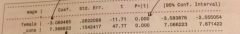
interpret this Stata output, which is based on the regression model reg wage female

Back 52

Note that the regression coefficient on "female" is statistically significant, meaning that gender has a statistically significant effect on the dependent variable wage. The regression coefficient on "female" means that on average, women in the sample earned $3.07 less per hour than men in the sample. The intercept means that the average (mean) wage of men in the sample was $7.36/hour. (note: this means that the mean wage of women in the sample was 7.36-3.07 = $4.29/hour)

Front 53

interpret this Stata output, which is based on the regression model reg wage female experience

Back 53

The regression coefficient on "female" means that women within the sample earn on average $2.66/hour less than men in the sample, holding experience constant. Note that the p-value for "female" is statistically significant, meaning there is a statistically sig. effect of gender on wage. The regression coefficient on "exper" means that a one-unit increase in experience is associated with a $0.65 increase in hourly wages, holding gender constant. The intercept means that a man with 0 experience has an average wage of $6.04/hour

Front 54

what if:
y = 1 if a person attends college, 0 otherwise
x1 = high school GPA
x2 = family income
and you get
yhat = b0 + b1x1 + b2x2
Then, what does
yhat =?
b1 =?
b2 =?

Back 54

yhat = the predicted probability of attending college
b1 = the change in the probability of attending college for each 1-unit increase in GPA, controlling for family income
b2 = the change in the probability of attending college for each 1-unit increase in family income, controlling for GPA

Front 55

what are problems with a regression model that has a dummy variable as the dependent variable?

Back 55

there are likely violations of the assumptions that we need for classical OLS. In particular, you will necessarily violate the following assumptions:
1. heteroskedasticity: there will be smaller variances as predicted values get close to 0 and 1
2. nonnormal error (i.e. the error term will not have a normal distribution)
3. nonlinearity: you might get predicted values OUTSIDE of the range of 0 to 1
for these reasons, there is a preference for logistic (logit) or probit analysis when the dependent variable is the dummy variable. But for exploratory purposes OLS regression is not bad at all (especially if the overall proportion of the dependent variable is between 0.2 and 0.8)

Front 56

what if you have a nominal variable with more than 3 categories? can you turn it into a dummy variable?

Back 56

yes, if you create a set of dummy variables to represent each of the 3 categories of the nominal variable

Front 57

if the nominal variable is "political party" and you have 3 categories, "democrat," "republican," and "other," what can you do to turn this into a dummy variable?

Back 57

create a set of dummy variables:
x1 = 1 if democrat, otherwise 0
x2 = 1 if republican, otherwise 0
x3 = 1 if other, otherwise 0
Note: they are all independent variables, b/c of the problems associated with treating dependent variable as a dummy variable

Front 58

how would you add these dummy variables to a regression model?

Back 58

you CANNOT add all three of the dummy variables to the regression model, b/c this would result in multicollinearity (b/c any one of the dummy variables would be a perfect linear function of the other two). As a result, you need to drop one of the dummy variables. The omitted dummy variable then becomes the reference category.

Front 59

which category/dummy variable should you drop?

Back 59

Stata usually drops the variable with the lowest number of cases from the regression model. The choice of the "omitted category" is not crucial, but judicious choice can facilitate interpretation. In some sense, the omitted category is the most important b/c it becomes the comparison. This is because the coefficient for a dummy variable is always a comparison (contrast) between that category and the omitted category. Note: when other independent variables are included in the model, the coefficient on the dummy variable is an adjusted difference in means

Front 60

if y = $ of political contributions in 2008, and
x1 = democrat
x2 = republican
and find
yhat = b0 + b1x1 + b2x2,
what does
b0=?
b1=?
b2=?

Back 60

b0 = the mean of the $ of political contributions in 2008 for individuals whose political affiliation is "other"
b1 = the difference in the mean political contributions between democrats and "others"
b2 = the difference in the mean political contributions between republicans and "others"

Front 61

what command in stata will create dummy variables for you based on the categories of a nominal variable?

Back 61

i.
ex. i.party will create a dummy variable for each value of the nominal variable "party"

Front 62

what is the coefficient for a dummy variable? (i.e how should it be interpreted)

Back 62

always a comparison (contrast) b/w that category and the omitted category. When other variables are included in the model, it is an adjusted difference in means

Front 63

if we add the variable x3 = income and estimate
yhat = b0 + b1x1 + b2x2 + b3x3
then what does
b0 =?
b1=?
b2 =?
b3 =?

Back 63

b0 = the average political contributions in 2008 of "Others" with an income of $0
b1 = the difference between the average political contribution of democrats and "others," controlling for income
b2 = the difference between the average political contributions of republicans and "others," controlling for income

Front 64

how can you change the omitted category in stata?

Back 64

reg cont ib3.party
where "cont" is the dependent variable
"i." tells stata to turn each category of the variable "party" into a dummy variable
"b3" tells stata to treat the 3rd category of the variable "party" as the omitted category

Front 65

what are the criteria for choosing the omitted category?

Back 65

1. don't choose a category with a small number of cases (induces near-extreme multicollinearity, which leads to high p-values for all dummy variables)...reason this is the case is b/c in calculating t-stat, divide difference by standard deviation divided by square root of n...so if n is very small, standard deviation will be large, meaning large denominator...this will result in smaller t-statistics and larger p-values...will likely conclude that there is not a relationship when there actually is a relationship (b/c will not reject H0 that no relationship)
2. choose a category that is a sensible standard of reference (if conflicts w/ criteria #1, go with criteria #1)
3. if there is a natural ordering to the categories, choose the lowest category (but if this conflicts w/ criteria #1, go with criteria #1)

Front 66

if you are doing a randomized experiment and have 1 control group and 2 treatment groups, which should you choose as the reference group if creating dummy variables for the 3 groups?

Back 66

The control group, b/c this is the sensible standard of reference/natural reference group

Front 67

what is invariant to the choice of omitted category?

Back 67

1. R-squared for the model
2. the coefficients of the other variables (outside of the set of dummy variables)
3. the differences between the coefficients of the dummy variables

Front 68

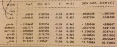
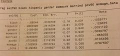
how would you interpret this Stata input for the regression of:
reg self90 ib3.race gender momwork married pov90 momage
where self90 = self-esteem level
where 1 = white non-hispanic, 2 = hispanic, and 3 = black?

Back 68

whites have a mean self-esteem level that is 0.68 units higher than blacks, controlling for all other variables in the model;
hispanics have a mean self-esteem level that 0.28 units lower than blacks, controlling for all other variables in the model; HOWEVER, there is not a statistically sig. diff. b/w the self-esteem levels of blacks and hispanics (p-value = 0.422), while there is a statistically sig. diff b/w self esteem levels of whites and blacks (p-value = 0.031)

Front 69

When dealing w/ a regression model that includes dummy variables as categories of an independent variable, what does the t-statistic for the slope coefficient of each dummy variable test?

Back 69

it tests the null hypothesis that there is no difference on the dependent variable between that category and the reference category (controlling for other variables in the regression)

Front 70

using this Stata output, how would we calculate the difference in the mean self-esteem level of blacks vs hispanics?

Back 70

If we want to know how whites compare to hispanics, we'd subtract the coefficient on whites from the coefficient on hispanics: 0.68 - (-0.28) = 0.96. This tells us that whites have self-esteem levels 0.96 units higher than hispanics. If want to know how hispanics compare to whites, we'd subtract the coefficient on hispanics from the coefficient on whites: -0.28 - 0.68 = -0.96. This tells us that hispanics have mean self-esteem levels 0.96 units lower than whites.

Front 71

how can you test whether two categories of a nominal variable differ in regards to a dependent variable y using Stata? (ex. does the mean self-esteem of blacks differ from that of hispanics)? How do you interpret the output?

Back 71

test category1=category2

ex:
test black=hispanic

If the Prob >F is above 0.05, you fail to reject the null, meaning you conclude that there is no evidence to challenge the null that there is no difference between the two categories regarding y

if the Prob > F is less than 0.05, you reject the null, meaning you conclude there is a statistically sig. difference b/w the two categories regarding y

Front 72

what formula can you use to manually calculate the test statistic?

Back 72

t = b4-b3/sqrt([variance of b4] + [variance of b3] - [2*covariance of b4&b3])

Front 73

how can you test whether a nominal variable transformed into multiple dummy variables has no overall (joint) effect on the dependent variable? How do you interpret the output?

Back 73

test (category1=0) (category2=0)
or
test category1 category2
or
testparm i.race

ex. if 1 = black, 2 = hispanic, and 3 = white non-hispanic and 3 is the omitted category, either

test (black=0) (hispanic=0)
or
test black hispanic
if told Stata to create dummy variables for variable "race" through command i.race, then:
testparm i.race

if Prob > F is more than 0.05, cannot reject the null that the nominal variable has no effect on y (i.e. joint effect of the dummy variables on y is 0)

if Prob > F is less than 0.05, reject the null hypothesis. The nominal variable race has a statistically significant effect on dependent variable y

Front 74

how can you run this test of the overall effect of the nominal variable on y by hand?

Back 74

1. run the regression model with the dummy variables to get R-squared (will call R^2L)
2. run the regression model without the dummy variables to get a second R-squared (will call R^2S)
3. Compute F = [(R^2L - R^2S)(n-K-1)]/[(1-R^L)(number of dummies put in model)]

Front 75

how do you perform an F test of the hypothesis that ALL of the coefficients in a regression model are equal to zero?

Back 75

in this case, R^2L = the R-squared for the model including all of the various independent variables
R^2S = the R-squared for the model without any independent variables, in which case R^2S will necessarily equal 0
F = [R^2L (n-K-1)]/[(1-R^2L)m]

Front 76

what is the relationship between multiple regression and analysis of variance (ANOVA)?

Back 76

-analysis of variance was designed for applications where you have an interval or ratio dependent variable and nominal (categorical) independent variables. nevertheless, there is an essential equivalence b/w ANOVA and multiple regression -- both are applications of the same linear model
-most ANOVAs can be done with multiple regression. Example: if dependent variable is self esteem and independent variable is race w/ 3 categories. We could test for a relationship b/w these 2 variables (self esteem and race) by means of a one-way ANOVA. The F-test for this ANOVA would be identical to the overall F-test in a multiple regression w/ 2 dummies representing race. So the following 2 commands will produce identical F-statistics:
reg self90 i.race
anova self90 race
-suppose we have another independent variable, gender, represented by a single dummy variable. If we add that to the regression equation, the test statistics for race and gender will be identical to those produced by a 2-way ANOVA, assuming no interaction b/w race and gender

Front 77

if we add an interval variable to the regression of race and gender on self-esteem, what will the test statistics be equivalent to?

Back 77

Analysis of Covariance

Front 78

does the standardized coefficient on a single, dichotomous dummy variable mean anything? what about the standardized coefficients on a set of dummy variables

Back 78

yes, the can help tell you the order of importance of dummy variables vs other variables in the model BUT you cannot interpret their numerical meaning (i.e. can't say 1 standard deviation increase in x results in ___ s.d increase/decrease in y)
as for sets of dummy variables, you can still compare their relative importance/difference from the omitted category, but can't interpret them nor compare them to other variables in the model

Front 79

what is the problem with using usual standardized coefficients to compare the effect of sets of dummy variables to the effect of other independent variables on y?

Back 79

1. there is only one conceptual variable, but several coefficients
2. each coefficient is a comparison with an omitted category

Front 80

how can you calculate a single standardized coefficient for a set of dummy variables?

Back 80

suppose we have y, x1, x2, x3, and x4. Suppose x1, x2, x3 are dummy variables representing a single nominal variable, and x4 is some other variable. We want a single standardized coefficient for x1, x2, and x3.
1. Run the regression in the usual way to get
yhat = b0 + b1x1 + b2x2 + b3x3 + b4x4

2. create a new variable z = b1x1 + b2x2 + b3x3, using the coefficients estimated in step 1

3. Do a second regression of y on z and x4. The standardized coefficient for z will be for the set of 3 dummy variables (if you're doing it right, the unstandardized coefficient for z should be 1.0 and both the standardized and unstandardized coefficients for x4 should be the same as in step 1)

Front 81

when else can you use the procedure described in the previous slide?

Back 81

Anytime you want a single standardized coefficient for a set of variables. For example
-several variables, all measuring some aspect of socio-economic status
-x and x^2
-x1, x2, and x1x2

Front 82

using the attached table, how would you create a standardized coefficient for the set of dummy variables within the nominal variable "race"?

Back 82

new variable z = b1(black) + b2(hispanic)
ie
new variable z = (-0.68)(black) + (-0.96)(hispanic)
in stata this would look like:
gen racecombo=-.68*black - .96*hispanic

reg self90 racecombo gender momwork married pov90 momage, beta

Front 83

what can we do if we want to include ordinal variables in multiple regression? (since ordinal variables aren't really appropriate for multiple regression)

Back 83

we can treat ordinal variables as nominal variables and represent them with dummies

Front 84

how would you turn the following ordinal variable into a nominal variable w/ a set of dummies?
x = level of security (where 3 = max security, 2 = medium security, and 1 = minimum security)

Back 84

create dummy variables for 2 of the 3 levels of security:
x3 = 1 if x=3, otherwise 0
x2 = 1 if x=2, otherwise 0

Front 85

if y = # of rule violations and you regress y on x2 and x3 to get
yhat = b0 + b2x2 + b3x3,
what does
b3 =?
b2 =?

Back 85

b3 = the difference in average rule violations between max security and min security
b2 = the difference in average rule violations b/w medium security and min security

Front 86

why can't you simply regress the ordinal variable, security level, on y?

Back 86

you could, but this imposes the assumption that the difference between min and medium security (in respect to rule violation) is the same as the difference between medium and max security (in respect to rule violation). You don't have any real basis for making that assumption. So, if the differences are not the same, then the coefficient on the ordinal variable will be the "average" of the two differences

Front 87

if you treat the ordinal variable as a nominal variable w/ dummies, how would you use stata to test the hypothesis of "no security effect" on "# of rule violations" (i.e. no effect of x on y)

Back 87

test x2 x3

Front 88

if you treat the ordinal variable as a nominal variable w/ dummies, how would you use stata to test the hypothesis the the difference between 1 and 2 (with respect to rule violations) is the same as the difference between 2 and 3?

Back 88

test x3 = 2*x2
this means that the effect of going from x1 to x3 is equal to 2x the effect of going from x1 to x2

Front 89

how would you interpret the output of the test of whether the interval b/w 1 and 2 is the same as interval between 2 and 3?

Back 89

if this test is significant (i.e. small p-value), we reject the "equal interval" hypothesis.

If it is not significant, and the only categories are 1, 2, and 3, then would just use the original ordinal variable w/o doing violence to the data (i.e. treat the ordinal variable as an interval variable, where each unit increase has same effect). If there are more than 3 categories, would need to do a different test to check for whether intervals b/w each of the categories are the same

Front 90

if you want to test more generally whether it is necessary to turn an ordinal variable into a set of dummy variables, what do you want to test for (conceptually)? (i.e. want to compare the "interval" [no dummies] model with the "nominal" model [dummies])

Back 90

you want to test the null hypothesis that each one unit increase in the ordinal variable has the same effect on y (i.e. "equal interval" hypothesis, where we are hypothesizing that all of the intervals are equal)

Front 91

what is one unfortunate consequence of breaking up a single variable into dummy variables?

Back 91

it results in a loss of parsimony and less statistical power (i.e. more likely to FAIL to reject the null [i.e. conclude no effect/relationship] when the alternative hypothesis is true)

Front 92

given the following regression line:

log(wage) = 0.2(experience) + 0.054(male) + 0.3(education)

where the variable "male" is a dummy variable (0= female, 1=male), how do you interpret the coefficient on male?

Back 92

males in the sample have an average wage that is 5.4% higher than the average wage of women in the sample, holding education and experience constant.

Front 93

given the following regression line:

log(wage) = 0.2(experience) - 0.054(black) -0.03(hispanic) + 0.3(education)

where the variable 'black' is a dummy variable (1 = black, 0 = otherwise) and the variable 'hispanic' is also a dummy variable (1 = hispanic, 0 = otherwise), and the third category (white) has been dropped, how do you interpret the coefficient on black?

Back 93

blacks in the sample had a mean wage that was 5.4% lower than whites in the sample, holding education and experience constant

Front 94

what do we do in stata to test the null hypothesis that each one unit increase has the same effect?

Back 94

perform a likelihood ratio test

1.perform regression w/ variable as an interval variable
2.use command "estimates store interval" to store the output of this first model
3. perform regression w/ variable as a nominal variable (w/ set of dummies)
4. use command "estimates store nominal" to store output of this second model
5. command: lrtest nominal interval

Front 95

how do you interpret the output of command "lrtest nominal interval"?

Back 95

if the Prob > chi2 is greater than 0.05, evidence that the simpler model (i.e. regression w/ the variable as an interval variable) is true. If it is less than 0.05, evidence that the more complex model (i.e. regression w/ the variable as a nominal variable w/ a set of dummies) is true. The null hypothesis is always that the simpler model is true and that each one-unit increase in the variable has the same effect on y

Front 96

in what situation can you use an F-test (as described earlier...involves looking at differences in R-squared) to test which model is better, interval or nominal?

Back 96

when the sample size is small. When it is large, you should use an likelihood ratio test

Front 97

what if you have a continuous interval variable but you suspect that particular levels of that variable matter more than just certain values of the variable...what can you do to test if this hypothesis is true?

Back 97

you can transform the continuous interval variable into a set of dummy variables and then test if the dummy variables add anything new to the regression model

Front 98

how could you turn the continuous interval variable "educe" (years of schooling) into a set of dummies?

Back 98

x1 = 1 if years of school is between 9 and 11, otherwise 0
x2 = 1 if years of school is 12, otherwise 0
x3 = 1 if years of school is between 13 and 15, otherwise 0
x4 = 1 if years of school is equal to or greater than 16, otherwise 0

Front 99

how would you test for whether treating educ as a set of dummies is more useful than treating it as a continuous interval variable?

Back 99

1.perform a regression of the dependent variable (lwage) on both educ and the dummy variables:

reg lwage educ x1 x2 x3 x4

2.perform a test of the joint effect of the dummy variables

test x1 x2 x3 x4

if the p-value is above 0.05, this means you should take the dummies out of the model and treat educ as a continuous interval variable. If the p-value is below 0.05, this means that the the dummies have a statistically signficant effect on lwage, meaning you should keep them in the model

Front 100

what are you really doing if you turn a continuous interval variable into a set of dummies?

Back 100

you are saying the relationship b/w this independent variable and y is NOT linear. You are also assuming that within the categories created by the dummy variables, everyone is the same in terms of the dependent variable (e.g. holding all other variables constant, there is no difference in lwage b/w a person with 9 years of school and a person with 10 years of school)

Front 101

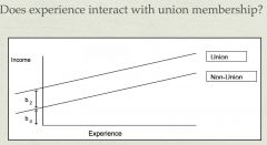
looking at this graph of the effect of experience on income by union membership, is there evidence for an interaction b/w union membership and experience? (i.e. is there evidence that union members and non-union members differ in terms of how experience affects their wages?)

Back 101

No, because the two lines are parallel. The top line represents the relationship b/w experience and income for union members. The bottom line represents the relationship b/w experience and income for non-union members. Although this graph illustrates that union members have higher wages than non-union members, the slopes of the 2 lines are the same, meaning the relationship b/w experience and income is the same for both groups

Front 102

what do b2 and b0 represent in this graph?

Back 102

b2 represents the difference between union and nonunion members in wages for people with 0 years of experience. Since the lines are parallel, the gap stays the same as experience increases.
b0 represents the wage of non-union members with 0 years experience

Front 103

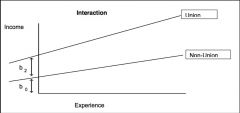
looking at this graph of the effect of experience on income by union membership, is there evidence for an interaction b/w union membership and experience? (i.e. is there evidence that union members and non-union members differ in terms of how experience affects their wages?)

Back 103

Yes, because the two lines are NOT parallel. Union members start out having higher wages than non-union members, and this difference increases as experience goes up. This means that the relationship b/w experience and income is not the same for both groups (a one-unit increase in experience has a greater effect on income for union members than for non-union members)

Front 104

how do you incorporate an interaction term between a dummy variable and a continuous interval variable into a regression model in stata?

Back 104

reg DV i.var1##c.var2 var3 var4

where "i." tells stata to create a dummy for each category of the variable and "c" signals to stata that the variable is a continuous variable

Front 105

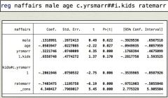
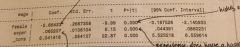
how would you interpret the output of this regression of "naffairs" (the number of affairs someone has) on independent variables that includes an interaction term b/w a dummy variable "kids" (1 = has kids, 0 = no kids) and a continuous interval variable "yrsmarr" (years married)?

Back 105

the coefficient on "yrsmarr" = for individuals w/o kids, a one unit increase in years married is associated with a 0.322 unit increase in number of affairs, controlling for other variables.
"1.kids" = for individuals who have been married for 0 years, those who have kids have 0.65 more affairs in past year than those who don't have kids.
kids#c.yrsmarr = the difference in the slope of number of affairs on years married between ppl with kids and ppl w/o kids (i.e. the difference in the main effect of years marriage on number of affairs b/w group w/ kids and group w/o kids). Note that this means that years of marriage has less of an effect on number of affairs for people with kids

Front 106

how do you calculate the main effect of years married on number of affairs for individuals with kids?

Back 106

you need to add (the main effect of of years married for individuals w/o kids) + (the interaction coefficient)
i.e. coefficient on "yrsmarr" + interaction coefficient. This would be 0.322 + (-0.206) = 0.116. So, this means, for individuals w/ kids, a one unit increase in years married is associated with 0.116 more affairs per year, controlling for other variables

Front 107

why would you include an interaction in the model instead of performing two separate models to describe how the variables affect the two groups differently?

Back 107

1. b/c running one regression gives you a direct test of whether or not the slopes are different for the 2 groups
2. if you have other independent variables, you can allow some slopes to differ and others to remain the same; that gives you a more parsimonious model, and thus higher power

that being said, separate tests might be desirable for ease of interpretation and reporting

Front 108

using stata, how can you perform two regressions to explore the relationship b/w x and y separately for 2 groups?

Back 108

bysort dummyvar: reg y x

ex. bysort union: reg wage exper

Front 109

how can you test whether the relationship b/w x and y are sig. different across the 2 groups?

Back 109

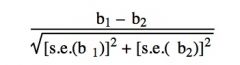
using the following test statistic:
where b1 = coefficient on x1 (first model)
b2 = coefficient on x2 (second model)
s.e.(b1) = standard error of b1
s.e.(b2) = standard error of b2

Front 110

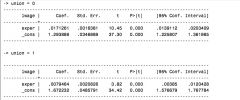
perform a test of difference in slope for the two groups, union and non-union, using the chart

Back 110

(0.017 - 0.0079)/sqrt([0.00163^2] + [0.00208^2])
t-stat = 3.5