Stats Exam 1

Front 1

Parameter

Back 1

is a numerical measurement describing some characteristic of a population

- population size of 241,472,385 is a parameter. because it is based on the entire population of all adults in the US

population; parameter

Front 2

Statistic

Back 2

is a numerical measurement describing some characteristic of a sample

sample; statisitc

Front 3

Statistic or a parameter?

in a AAA Foundation for Traffic safety survey, 21% of the residents said that they recently texted or e-mailed while driving

Back 3

Statistic: sample of the population not the whole population

Front 4

Sample

Back 4

is a subcollection of members selected from a population

the objective is to use the sample data as a basis for drawing a conclusion about the population of all adults, and methods of statistics are helpful in drawing such conclusions

Front 5

Quantitative Data

Back 5

( or numerical) data consists of numbers representing counts or measurements

- the ages in years of survey participents

Front 6

Qualitative Data

Back 6

(or Categorical/attribute) data consists of names or labels that are not numbers representing counts or measurements

- party affiliation, jersey numbers

Front 7

Statistic or parameter?

a study was conducted of all 2223 passengers aboard the titanic when it sank.

Back 7

Parameter: the whole population of all the passengers, not a sample of some of them

Front 8

Simple Random Sample

Back 8

a sample of n subjects is selected in such a way that every possible sample of the same size n has the same chance of being chosen

Front 9

Random Sample

Back 9

each member of the population has an equal chance of being selected

- computers are often used to generate random telephone numbers

Front 10

Systematic Sampling

Back 10

select some starting point, then select every kth (such as every 50th) element in the population

Front 11

Convenience Sampling

Back 11

use results that are easy to get

Front 12

Stratified Sampling

Back 12

subdivide the population into at least 2 diff subgroups (or strata) so that subjects within the same subgroup share the same characteristics (such as gender or age bracket) then drawa sample from each subgroup

Front 13

Cluster Sampling

Back 13

divide the population into sections (or clusters), then randomly select some of those clusters, and then choose all members from those selected clusters

Front 14

Simple random sample?

every 100oth pill is selected and tested

Back 14

not a simple random sample because every 1000th pill is selected, some samples have no chance to of being selected.

for example, two consecutive pills has no chance of being selected and this violates the requirement of a simple random sample

Front 15

page 37 #9

Front 16

How are graphs able to deceive?

Nonzero axis

Back 16

Nonzero axis: exaggerates the difference and can create a false impression

Front 17

How are graphs able to deceive?

pictographs

Back 17

Pictographs: data that are one dimensional in nature (such as budget amts) are often depicted with two or three dimensional objects. pictographs can create flase impressions that grossly distort differences by using these simple principles of basic geometry:

(1) when you double each side of a square, the area doesn't merely double; it increases by a factor of four

(2) cube sides doubled: area increases by a factor of 8

Front 18

Normal Distibution

Back 18

(1) the frequencies start low, then increase to one or two high frequencies, and then decrease to a low frequency

(2) the distibution is approximately symmetric, with frequencies preceding the maximum being roughly a mirror image of those that follow the maximum

Front 19

Relative Frequency Distribution

Back 19

in which each class frequency is replaced by a relative frequency (or proportion) or a

percentage

frequency for a class/sum of all frequencies

x 100%

Front 20

Class boundaries

Back 20

are the numbers used to seperate the classes, but without gaps created by class limits

50-69

70-89

90-109

110- 129

130-149

49.5,69.5, 89.5, 109.5,129.5,149.5

Front 21

Class width

Back 21

is the difference between two consecutive lower class limits (or two lower class boundaries) in a frequency distribution

50-69

70-89

20 class width

Front 22

frequency distribution

Back 22

shows how data are partitioned among several categories (or classes) by listing the categories along with the number (frequency of data values in each of them

Front 23

a complete list of all 241,424 adults in the US is compiled and every 150th name is selected

Back 23

Systematic

Front 24

a complete list of all 241,424 adults in the US is compiled and 1500 adults are randomly selected from this group

Back 24

Random

Front 25

the US is partitioned into regions with 100 adults in each region. then 15 of those regions are randomly selected

Back 25

cluster

Front 26

The US is partitioned into 150 regions with approximately the same number of adults in each region. then 10 people are randomly selected from each of the 150 regions

Back 26

stratisfied

Front 27

a survey is mailed to 10,000 randomly selected adults, and 1500 response's were used

Back 27

convenience

Front 28

Why construct a frequency distribution?

Back 28

(1) so that we can summarize large data sets

(2) so that we can analyze the data to see the distribution and identify outliers

(3) so that we have a basis for constructing graphs

Front 29

Cumulative Frequency Distribution

Back 29

use original frequencies i.e. 2,33,35,7,1

Cumulative, add up like this:

2+33= 35

2+33+35= 70

70+7=77

77+1=78

Front 30

the presence of gaps in frequency can suggest....

Back 30

that the data are from two or more different populations

Front 31

Histogram

Back 31

Is a graph consisting of bars of equal width drawn adjacent to each other (unless there are gaps in the data). The horizontal scale represents classes of quantitative data values and the vertical scale represents frequencies. The heights of the bars corresponds to the frequency values

Front 32

the distribution of data is skewed if...

Back 32

it is not symmetric and extends more to one side than the other

Front 33

Skewed to the right

Back 33

positively skewed:

have a longer right tail:

more common than data skewed to the left because it's often easier to get exceptionally large values than values that are exceptionally small.

Front 34

example of annual incomes and where they are skewed

Back 34

with annual incomes, impossible to get values below zero, but there are a few people who earn millions or billions each year. Annual incomes tend to be skewed to the right

Front 35

skewed to the left

Back 35

negatively skewed:

have a longer left tail

Front 36

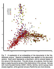
Scatterplot

Back 36

or scatter diagram

plot of paired (x, y) quantitative data with a horizontal x-axis and a vertical y-axis:

the pattern of the plotted points is often helpful in determining whether there is a correlation between two variables

Front 37

Time-Series Graph

Back 37

a graph of time-series data which are quantitative data that have been collected at different points in time, such as yearly or monthly

Front 38

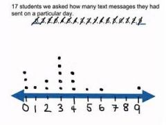
Dot-Plot

Back 38

consists of a graph in which each data value is plotted as a point along a horizontal scale of values

Front 39

Stemplot

Back 39

represents quantitative data by separating each value into two parts; the stem (left most digit) and the leaf (rightmost digit)

Advantage:

(1)we see the distinction of data while keeping the original data values

(2) constructing a stemplot is a quick way to sort data, which is required for some statistical procedures (such as finding a median)

Front 40

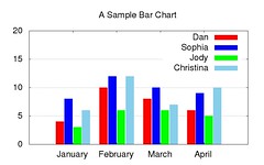
Bar Graph

Back 40

uses bars of equal width to show frequencies of categories or categorical (qualitative) data

Vertical side: represents frequencies or relative frequencies

Horizontal: identifies categories of qualitative data

Front 41

Principles of Tufte

Back 41

1. small data sets of values of 20 or fewer; use a table instead of a graph

2. a graph of data should make us focus on the true nature of the data, not on other elements, such as eye catching designs

3. do not distort data; construct a graph to reveal the true nature of the data

Front 42

Pie Chart

Back 42

a graph that depicts categorical data as slices of a circle, in which the size of each slice is proportional to the frequency count for the category

Front 43

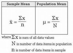
Mean

Back 43

of a data set is the measure of center found by adding the data values and dividing the total by the number of data values

Front 44

Important properties of Mean

Back 44

1. sample means drawn from the same population tend to vary less than other measure of center

2. the mean of the data set uses every data value

3. a disadvantage of the mean is that just one outlier can change the value of the mean significantly

(it is not a resistant measure of center)

Front 45

Σ denotes the sum of a data set

x the variable usually used to represent the individual data set

n represents the number of data values in a

sample

N represents the number of data sets in a

population

x ̃=εx/N is the mean of a set of sample values

µ=Σ_x/N is the mean of all values in a population

Front 46

Median

Back 46

"middle value" half of the values in a data set are less than the median and half are greater than the median.

Front 47

Mode

Back 47

of a data set is the value that occurs with the greatest frequency

Bimodal: 2 modes

Multimodal: more than two modes

No mode: when no data value is repeated

Front 48

Midrange

Back 48

of a data set is the measure of center that is the value midway between the maximum and the minimum values in the original data set.

Max +Min/2

Front 49

round off rules

Back 49

for the mean, median and midrange, carry one decimal place than is present in the original set of values

for the mode, leave the value as is (because values of the mode are the same as some of the original data value)

Front 50

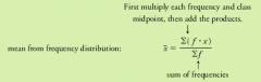
Mean for frequency distribution

Back 50

x ̃=(∑(f ̇⋅x ̇ )/(∑f)

Frequency x Class midpoint = F x X

Add up all frequencies of Ef and add up all E(FxX)

Divide E(FxX) by Ef to get the mean from frequency distribution

Front 51

Measures of Variation

Back 51

1. range

2. standard deviation

3. variance

Front 52

Range

Back 52

of a data set is the difference between the maximum data value and the minimum data value

- very sensetive to outliers

Front 53

standard deviation

Back 53

*most commonly used in statistics

of a set of sample values, denoted by s, is a measure of how much data values deviate away from the mena.

Front 54

Important properties of Standard Deviation

Back 54

(1) the SD is a measure of how much data values deviate away from the mean

(2) the value of the standard deviation, s, is usually positive. it is zero only when all values of the data values are the same number. NEVER negative

(3) the value of the standard deviation can increase dramatically with the inclusion of one or more outliers

(4) the units of the SD s (such as minutes, feet, pounds) are the same as the units of original data values

(5) he sample standard deviation s is a biased estimator of the population standard deviation denoted by σ

Front 55

three concepts that can help us determine and interpret values of standard deviation

Back 55

(1) the range rule of thumb

(2) the empirical rule

(3) Chebyshev's theorem

Front 56

Range rule of thumb

Back 56

tool for interpreting Standard Deviation:

It is based on the principle that for many data sets, the vast majority (such as 95%) of sample values lie within 2 Standard Deviations of the mean.

Minimum usual value = (mean) - 2 x (standard deviation)

Max usual value = (mean) + 2 x (standard devaition)

Front 57

Estimating a value of the standard devaition

Back 57

s ≈ range/4 with range being the max-min

Front 58

Variance

Back 58

of a set of values is a measure of variation equal to the square of the standard deviation

s^2 = sample variance

σ ^2 = population variance

Front 59

Important properties of Variance

Back 59

(1) the units of variance are the squares of the units of the original data. if the values are in feet, the varaince will have units of ft^2

(2) the value of variance can increase dramatically with the inclusion of one or more outliers

(3) the value of variance is usually positive. it is zero only when all of the data values are the same number

(4) the sample variance s^2 is an unbiased estimator of the population variance σ ^2

Front 60

don't forget units of measurement after each data!!!!!