Structural Geology Test 3

Front 1

Stress vs. strain 1

Back 1

1. Stress is defined as a force that can cause a change in an object or a physical body while strain is the change in the form or shape of the object or physical body on which stress is applied.

2 . Stress can occur without strain, but strain cannot occur with the absence of stress.

3. Stress can be measured and has a unit of measure while strain does not have any unit and, therefore, cannot be measured.

Front 2

Stress vs. strain 2

Back 2

1. In the field you never see stress, we only see the results of stress as it deforms minerals.

2. Even if we were to sue a strain gauge to measure in-situ stress in the rock, we would measure the stress itself.

3. We would measure the deformation of the strain gauge and use that to infer the stress.

Front 3

Stress vs. strain 3

Back 3

1. Strain is an object’s response to stress while stress is the force that can cause strain in an object.

Front 4

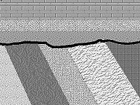
Ideal shear zone 1

Back 4

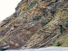
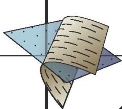
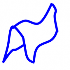
1. Ideal shear zone (ductile shear zone) has planar and parallel boundaries outside of which there is no strain; in reality, boundaries typically are gradational.

Front 5

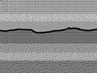
Ideal shear zone 2

Back 5

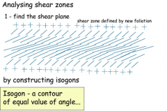
Analyze shear zones?

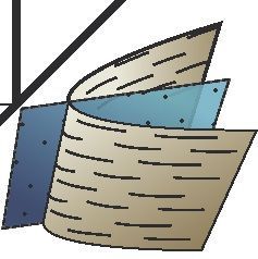
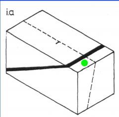
1. Find the shear plane: Shear planes are defined by new foliation; by constructing isogons (a contour of equal value of angle)

Front 6

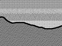
Ideal shear zone 3

Back 6

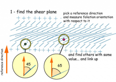
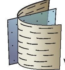
2. Find the shear plane: Pick a reference direction and measure foliation orientation with respect to it and finds others with same value then link up.

Front 7

Ideal shear zone 4

Back 7

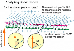
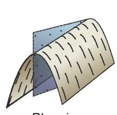
4. Once shear plane is found, we construct a profile 90 degrees to shear plane and measure the strain along it, so shear runs E to W across the screen, and measure angle relative to reference direction.

Front 8

Ideal shear zone 5

Back 8

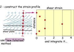
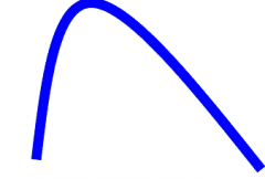
4. Construct the strain profile using the shear strain formula (y= tanφ), using the and integrate it into a distance (Y) vs shear strain graph (X)

Front 9

Ideal shear zone 6

Back 9

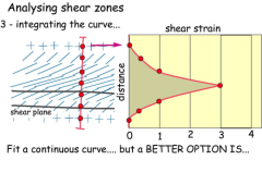
5. Once you integrate the curve, it should fit in a continuous curve BUT a better option is... to use a stepped graph.

- Note that peak strain of zone; example is symmetric.

Front 10

Ideal shear zone 7

Back 10

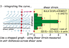
6 .The stepped graph: using shear strain measured in unit distances across shear zone.

Front 11

Ideal shear zone 8

Back 11

1. We assume shear strain in this model.

2. Rocks encountered in shear zones:

- Uncohesive fault rocks (e.g. fault gouge, fault breccia, and foliated gouge).

- Cohesive fault rocks (crush breccias and cataclasites).

- Glassy pseudotachylites.

- Foliated mylonites (phyllonites)

- Striped gneiss.

Front 12

Rheology variables 1

Back 12

1. Rheology is the study of the flow of matter, primarily in a liquid state, but also as 'soft solids' or solids under conditions in which they respond with plastic flow rather than deforming elastically in response to an applied force.

Front 13

Rheology variables 2

Back 13

1. Lithology: a rock unit is a description of its physical characteristics visible at outcrop, in hand or core samples or with low magnification microscopy, such as color, texture, grain size, or composition.

2. Competence refers to the degree of resistance of rocks to either erosion or deformation in terms of relative mechanical strength.

3. Incompetent rock: tend to form lowlands and are often poorly exposed at the surface, incompetent beds tend to deform more plastically.

4 . Competent rock: are more commonly exposed at outcrop as they tend to form upland areas and high cliffs or headlands, where present on a coastline. During deformation competent beds tend to deform elastically by either buckling or faulting/fracturing.

Front 14

Rheology variables 3

Back 14

1. Pressure: force per unit area. Pressure is exerted by liquids and gases and is equal in all directions.

2. Pressure solution or pressure dissolution is a deformation mechanism that involves the dissolution of minerals at grain-to-grain contacts into an aqueous pore fluid in areas of relatively high stress and either deposition in regions of relatively low stress within the same rock or their complete removal from the rock within the fluid confining pressure, pore fluid press and effective stress.

2. Confining pressure pressure applied equally on all surfaces of a body. For example, a diver below the surface of the ocean is subject to water pressure in all directions. In the earth we say use the term confining pressure when we mean that rock stress is equal in all directions.

Front 15

Rheology variables 4

Back 15

1. Temperature: An increase in the temperature of a rock generally depresses yield strength, enhances ductility greatly, and lowers ultimate strength.

2. Some rocks are more sensitive to the effects of temperature than others.

3. Igneous rocks are less affected by modest increases in temperature than sedimentary rocks; they are more at home in high-temperature environments.

4. COLD & STRONG VS. HOT & WEAK

Front 16

Rheology variables 5

Back 16

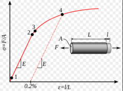
1. Strain rate: A rock can be forced to deform plastically at comparatively low levels of stress if the rate of loading is slow.

2. Creep is the strain produced in experiments of long duration under differential stresses that are well below the rupture strength of the rock.

3. Results of the tests produce consistent plots, like those shown in Figure 3.6

4. As soon as the load is applied, the rock experiences an elastic deformation.

5. This is followed by three distinctive kinds of mechanical response, called primary, secondary, and tertiary creep.

6. FAST vs. SLOW (think silly putty experiment)

Front 17

Rheology variables 6

Back 17

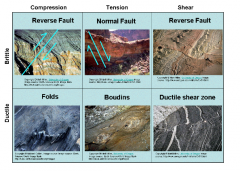
1. Time: a certain amount of time is required for chemical reactions to equilibrium.

2 . SLOW & DUCTILE: a rock subject to differential stress at high temperature or slow rate of deformation will flow like putty. This type of deformation often leads to folds in the Earth.

3. FAST & BRITTLE: a rock subject to a large differential stress at low temperature or high rate of deformation will fracture, crack, or shatter like glass. This type of deformation often leads to faults and earthquakes in the Earth. The differential stress at which a rock fractures is called its brittle strength. As differential stress often increases from zero, a rock will deform elastically before reaching its brittle strength.

Front 18

Rheology variables 7

Back 18

1. Pre-existing weaknesses and Structural "inheritance": a key factor to understand the tectonicevolution and structural deformation pattern of the lithosphere. Inparticular, successive rifting events often occurred in regions whereoceanic crust is now forming. The multiple rifting events may have thesame kinematics (rift and divergence trends) or different ones.

2. ISOTROPIC; When the properties of a material vary with different crystallographic orientations.

3. ANISOTROPIC: when the properties of a material are the same in all directions,

4. Reactivation of structures often occurs when displacements are repeatedly focused along well-defined features such as faults, shear zones, or lithological contacts.

Front 19

Rheology variable 8

Back 19

1 . Size: The Himalayas , Sand, Silly Putty, and Honey

Front 20

Ductile deformation 1

Back 20

1. Ductile deformation is when at higher temperatures and pressures, many rocks flow in response to stress.

2. Ductile deformation is not recoverable must result from permanent changes in material.

3. Ductile deformation mechanisms- higher temperature, higher pressure, slower strain rate, lower fluid pressure.

Front 21

Ductile deformation 2

Back 21

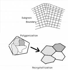
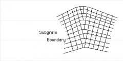
1. Recovery is the process of returning the crystal to its original undeformed state. If dislocations pile-up in a line perpendicular to their direction ofmotion then a subgrain boundary is formed.

2. Recrystallization takes place when high angle grain boundaries sweep through the crystal. The high angle grain boundaries sweep outmany of the defects in the crystal. The process of normal grain growth tries to reduce grain boundary tension by putting grains next to each other with the smallest energy.

Front 22

Ductile deformation 3

Back 22

1. Polygonization is the process where edge dislocations climb by atom or vacancy diffusion and glide to low-energy polygonal networks. Here the subgrain boundaries are at very small angles to neighbors.

2. Recrystallization takes place when high angle grain boundaries sweep through the crystal. The high angle grain boundaries sweep out many of the defects in the crystal. The process of normal grain growth tries to reduce grain boundary tension by putting grains next to each other with the smallest energy.

Front 23

Ductile deformation 3

Back 23

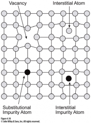
1. Point defects are where an atom is missing or is in an irregular place in the lattice structure.

2. Point defects can be composed of:

- impurities: foreign atom in crystals tructure,

- vacancies: atom is missing from crystal lattice, resulting in a hole,

- interstitials: foreign atom in spaces between atoms.

Front 24

Ductile deformation 4

Back 24

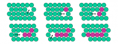
1. Typically, crystals contain more vacancies, at higher temperatures purple atoms move by jumping into adjacent vacancy.

2. Note that atoms and vacancies diffuse in opposite direction applied stress creates gradient in vacancy concentration; atoms migrate down gradient away from applied stress causing material to flow.

Front 25

Ductile deformation 5

Back 25

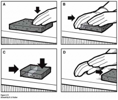
1. Dislocation: linear array of atoms that bounds an area incrystal that has slipped relative to rest of crystal.

2. Envision with sponge experiment

- wring out wet sponge,

- place on countertop,

- put hand on top half,

- exert pressure so halfbelow hand won’t slide,

- push on end of spongewith other hand

- countertop = slip plane

- sponge = crystal lattice

3. Line separates slipped sponge from unslipped sponge = dislocation

Front 26

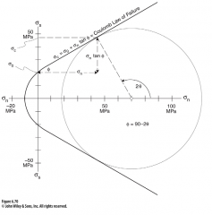
Byerlee's law

Back 26

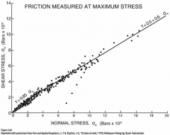
1. Law describing conditions under which an existing fracture will slip is a modification of the Coulomb law of failure, since a fractured rock has no cohesion, the term for cohesive strength is removed, leaving:

- σc = tanφ (σn), (σ = sigma and φ = phi)

2. Byerlee found that the coefficient of sliding friction,

- μf = tanφf, (μ = mu and φ= phi),

is the same for almost all rocks: at low magnitude of confining pressure,

- μf = 0.85,

and the angle of sliding friction is ~40 degrees, for moderate to higher confining pressure the angle is ~35 degrees.

Front 27

Brittle-ductile transition 1

Back 27

1. The brittle-ductile transition zone is the strongest part of the Earth's crust.

2. For quartz and feldsparrich rocks in continental crust this occurs at an approximate depth of 13–18 km (roughly equivalent to temperatures in the range 250-400°C).

3. At this depth rock becomes less likely to fracture, and more likely to deform ductilely by creep.

Front 28

Brittle-ductile transition 2

Back 28

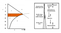
1. Brittle elastic and frictional processes dominate.

2. Brittle-ductile Transition Zone

3. Crystaplastic processes dominate.

4. Strength increases linearly with confining pressure (& depth)

5. Strength decreases exceptionally with temperature (& depth)

6. Strength

7 . Depth (km)

Front 29

Importance of T-deformation mechanisms

Back 29

1. Faulting within a three dimensional strain environment Coulomb theory predicts faults should form in conjugate sets Faults in nature sometimes display two pairs of conjugate fault sets must include different amounts of strain in three directions (3D instead of plane strain).

Front 30

Mohr Failure Envelope 1

Back 30

1. A means by which two stresses acting on a plane of know orientation can be plotted as the components of normal and shear stresses (derived separately from each of the two stresses).

2. An elegant way to determine the shear andnormal stresses for a pair of stresses oriented obliquely to the planein question. The Mohr circle allows you to quickly read this forplanes of any orientation.

3. It also makes it easy to visualize mean stress and differences instress, or deviatoric stress and relate these to deformation.

Front 31

Mohr Failure Envelope 2

Back 31

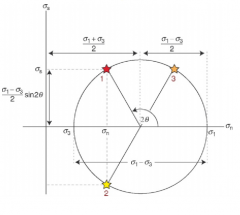
1. Stress Equations: Two perpendicular stresses oriented at anyangle to a plane.

2. Normal Stress:

- σn = [(σ1 + σ3) / 2] + [(σ1 - σ3) / 2] x cos 2Θ

3. Shear Stress

- σs = [(σ1 - σ3) / 2] x sin 2Θ

4. Theta is the angle between the maximum stress and the poleto the plane the stresses are acting upon.

Front 32

Mohr Failure Envelope 3

Back 32

1. Mean or average stress.

2. Deviatoric stress.

3. Differential stress.

Front 33

Mohr Failure Envelope 4

Back 33

1, Tensile stress: necessary to cause tensile failure represented by apoint, the tensile strength, on σn axis to left of σs.

2. From Griffith crack theory, depends on flaws..highly variable.

3. Tensile strength (experiments show less than compressive strength).

Front 34

Mohr Failure Envelope 5

Back 34

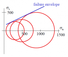
1. Mohr circles that defines tress states where samples fracture(critical stress states)together define the failure envelope for a particular rock.

2. Failure envelope is tangent to circles of all critical stress states and is a straight line, can also draw failure envelope in negative quadrant for σs (mirror image about σn axis).

3. This straight line corresponds to Coulomb fracture criterion (theta = 60).

Front 35

Mohr Failure Envelope 6

Back 35

1. High confining pressures: begin to have plastic deformation;

- cannot have “failure” envelope, implies brittle.

- can approximate “yield” envelope…sample yields plastically.

2. Two parallel lines that parallel σn axis known as Von Mises criterion (theta = 45) which is independent of differential stress.

3. Pore-fluid pressure shifts everything to the left.

Front 36

Coulomb’s Fracture criterion 1

Back 36

1. σc = tanφ (σn)

2. σ or sigma (symbol for stress)

3. σn is the magnitude of the normal stress

4. σc is closing stress

5. phi or φf is the angle of sliding friction (slope of the envelope the tangent of φf is the coefficientof sliding friction μf= tan φf)

Front 37

Stress cube 1

Back 37

1. Stress acts on every surface that passes through the point, we can use three mutually perpendicular planes to describe the stress state at the point, which we approximate as a cube.

2. Each of the three planes as one normal component & two shear components.

3. Therefore, 9 components necessary to define stress at a point, 3 normal and 6 shear.

4. This is the stress tensor remember, a vector, which represented by 3 coordinates in a Cartesian reference frame (x, y, z, this is a matrix with 3 components stress at a point has nine component, this is a matrix with 9 components (second-rank tensor).

Front 38

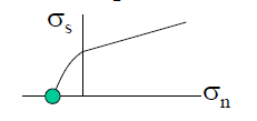
Strength on stress vs strain diagram 1

Back 38

1. A yield strength or yield point of and materials science as the stress at which a material begins to deform plastically.

2. Prior to the yield point the material will deform will return to its original shape when the applied stress is removed. Once the yield point is passed, some fraction of the deformation will be permanent and non-reversible.

3. In the three-dimensional space of the principal stresses (σ1, σ2, σ3), an infinite number of yield points form together a yield.

Front 39

Strength on stress vs strain diagram 2

Back 39

Stress–strain curve showing typical yield behavior for nonferrous alloys. Stress (σ) shown as a function of strain (e).

1. True Elastic limit

2. Proportinality limit

3. Elastic limit

4. Offset yield strength

Front 40

Strength on stress vs strain diagram 3

Back 40

1. True elastic limit The lowest stress at which dislocations move. This definition is rarely used, since dislocations move at very low stresses, and detecting such movement is very difficult.

2. Proportionality limit Up to this amount of stress, stress is proportional to strain (Hooke's law), so the stress-strain graph is a straight line, and the gradient will be equal to the elastic modulus of the material.

3. Proportionality limit Up to this amount of stress, stress is proportional to strain (Hooke's law), so the stress-strain graph is a straight line, and the gradient will be equal to the elastic modulus of the material.

4. A yield strength or yield point of and materials science as the stress at which a material begins to deform plastically

Front 41

Andersonian fault theory 1

Back 41

1. Relies on one fundamental assumption: The Earth’s surface is a principal plane of stress (a free surface that can’t support shear).

2. This, together with = 30°, means only normal‐slip, strike‐slip, and thrust faults should be able to form near the Earth’s surface.

3. Does not account for Oblique-slip faults and Dip-slip faults.

Front 42

Andersonian fault theory 2

Back 42

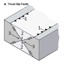
Thrust-slip faults

1. 30°

2. σ3

3. σ1

Front 43

Andersonian fault theory 3

Back 43

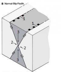
Normal-slip fault:

1. 60°

2. σ3

3. σ1

Front 44

Andersonian fault theory 4

Back 44

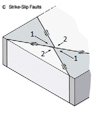
Strike-slip fault:

1. σ3

2. σ1

Front 45

Components of Fault Displacement 1

Back 45

1 . Net slip: Or total slip is the direct distance measured between the two originally adjacent points.

2 . Dip slip: Measure of distance between the line of strike and the adjacent point.

3. Strike slip: Measure of distance between the point and where dip slip intersects strike.

Front 46

Components of Fault Displacement 2

Back 46

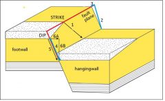
4. Strike separation: Component of separation parallel to strike.

5. Dip separation: Component of separation parallel to dip.

6A. Heave: Horizontal component of separation.

6B. Throw: Vertical component of dip separation.

Front 47

Piercing Points 1

Back 47

Piercing point is defined as a feature that is cut by a fault, then moved apart. The points we adjacent before faulting.

Front 48

Types of Unconformities 1

Back 48

1. Angular unconformity: Are those where an older package of sediments has been tilted, truncated by erosion, and than a younger package of sediments was deposited on this erosion surface.

Front 49

Types of Unconformities 2

Back 49

1. Disconformity: The surface of a division between parallel rock strata, indicating interruption of sedimentation.

Front 50

Types of Unconformities 3

Back 50

1. Non-conformity: Are unconformities that separate igneous or metamorphic rocks from overlying sedimentary rocks. They usually indicate that a long period of erosion occurred prior to deposition of the sediments.

Front 51

Fold classification by orientation of axial plane and fold axis 1

Back 51

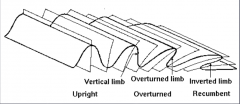
1. Axial plane: Folds can be classified based on the dips of limbs and the axial plane. The spectrum of fold orientations generally corresponds to a gradient in strain.

Front 52

Fold classification by orientation of axial plane and fold axis 2

Back 52

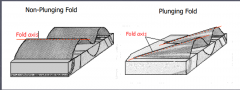
1. Fold axis: Folds can be classified based on the orientation of the fold axis. Horizontal/Non-Plunging and Plunging (Shallow, Moderate, Steep, Vertical, North, South, East, West, etc.)

Front 53

Fold profile view 1

Back 53

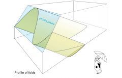
1. A folded surface is fully described in a plane perpendicular to the fold axis.

2. The profile of a fold is the section drawn perpendicular to the fold axis and its axial surface; this contrasts with a geological section which is normally drawn in a vertical plane.

Front 54

Fold Types 1

Back 54

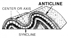
1. Anticline: linear, strata normally dip away from axial center, oldest strata in center.

Front 55

Fold Types 2

Back 55

2. Syncline: linear, strata normally dip toward axial center, youngest strata in center.

Front 56

Fold Types 3

Back 56

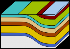
3. Monocline: linear, strata dip in one direction between horizontal layers on each side

Front 57

Fold Types 4

Back 57

1. Chevron: angular fold with straight limbs and small hinges.

Front 58

Fold Types 5

Back 58

1. Recumbent: linear, fold axial plane oriented at low angle resulting in overturned strata in one limb of the fold.

Front 59

Fold Types 6

Back 59

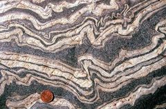
1. Ptygmatic: Folds are chaotic, random and disconnected. Typical of sedimentary slump folding, migmatites and decollement detachment zones.

Front 60

Fold Types 7

Back 60

1. Parasitic: short wavelength folds formed within a larger wavelength fold structure - normally associated with differences in bed thickness.

Front 61

Fold Types 8

Back 61

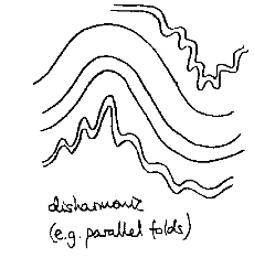
1. Disharmonic: Folds in adjacent layers with different wavelengths and shapes.

Front 62

Fold Types 9

Back 62

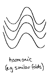
1. Harmonic: fold which maintains its geometric form, integral wavelength, and symmetry throughout a sequence of layers

Front 63

Parts of a fold 1

Back 63

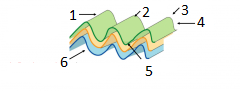
1. Hinge line: where curvature is the greatest.

2. Crest.

3. Hinge

4. Limb

5. Trough

6. Inflection point: where sense of curvature changes.

Front 64

Parts of a fold 2

Back 64

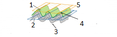
1. Enveloping surface (antiform / connect crest).

2. Enveloping surface (synform / connect troughs).

3. Synform (Valley) or Synclinorium (Regional).

4. Antiform (Hill) or Anticlinorium (Regional)

5. Enveloping surface: Defines limit of fold.

Front 65

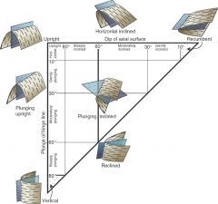
Fleuty's Fold Classification 1

Back 65

Front 66

Fleuty's Fold Classification 2

Back 66

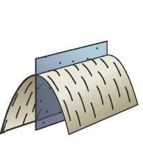
1. Upright: Dip of axial surface is upright or plunge of hingeline is horizontal.

Front 67

Fleuty's Fold Classification 3

Back 67

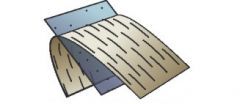
2. Horizontal inclined: Moderately inclined axial surface and horizontal hingeline.

Front 68

Fleuty's Fold Classification 4

Back 68

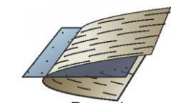
3. Recumbent: Dip of axial surface recumbent and plunge of hingeline is horizontal, less than 10 degrees.

Front 69

Fleuty's Fold Classification 5

Back 69

4. Plunging inclined: Dip of axial surface at 60 degrees and plunge of hingeline at 30 degrees.

Front 70

Fleuty's Fold Classification 6

Back 70

5. Reclined: Dip of axial surface at 60 degrees and plunge of hingeline at 60 degrees.

Front 71

Fleuty's Fold Classification 7

Back 71

6. Vertical: Dip of axial surface vertical and plunge of hingeline is upright, more than 80 degrees.

Front 72

Fleuty's Fold Classification 8

Back 72

7. Plunging upright: Gently plunging hingeline and upright dip of axial surface.

Front 73

Four basic patterns of fold superposition 1

Back 73

Superimposed fold: Generations of folds that happen after the diagenesis of the bed and its first folding by tectonic events. A superposed fold is younger than structure it folds.

Front 74

Four basic patterns of fold superposition 2

Back 74

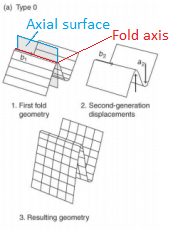
1. Type 0: Cannot see as interference type; axial surfaces parallel.

Front 75

Map patterns of fold interface folding 3

Back 75

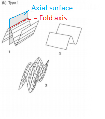
2. Type 1: “Dome-and-basin” structure, egg-carton, axial surfaces normal.

Front 76

Map patterns of fold interface folding 4

Back 76

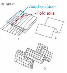
3. Type 2: Most difficult to visualize; “mushroom.”

Front 77

Map patterns of fold interface folding 5

Back 77

4. Type 3: “Refolded folds” (all types are refolded)

Front 78

Modes of Fractures according to tip line 1

Back 78

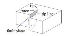
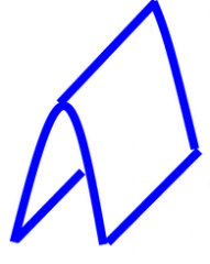
1. Tip line: line that separates slipped from unslipped rock; (where fault displacement goes to zero) tip line is a closed loop.

Front 79

Modes of Fractures according to tip line 2

Back 79

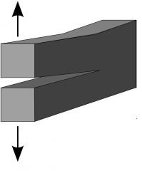
1. Opening mode: Mode I fracture, a tensile stress normal to the plane of the crack .

Front 80

Modes of Fractures according to tip line 3

Back 80

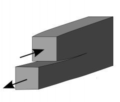
2. : Sliding mode: Mode II fracture, A shear stress acting parallel to the plane of the crack and perpendicular to the crack front.

Front 81

Modes of Fractures according to tip line 4

Back 81

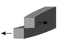
3. Tearing mode: Mode III fracture, a shear stress acting parallel to the plane of the crack and parallel to the crack front.

Front 82

Younging Direction 1

Back 82

1.To know if beds we overturned.

2. Tectonic history of the bed.

3. Mineral exploitation.

4. Kinematic information.

Front 83

Cylindrical folds vs Non-cylindrical folds 1

Back 83

1. Cylindrical Folds: Straight hinge lines and contain fold axes.

Front 84

Cylindrical folds vs Non-cylindrical folds 1

Back 84

2. Non- Cylindrical Folds: Curved hinge lines and does not contain fold axes.

Front 85

Symmetric vs asymmetric folds 1

Back 85

1. Symmetric: Limbs have equal dips.

Front 86

Symmetric vs asymmetric folds 2

Back 86

2. Asymmetric: Unequal limb dip angles.

Front 87

Fault Recognition 1

Back 87

1. Features of faults themselves: Fault rocks (i.e. Fault Breccia ect.) or Slickensides, slickenlines etc.

Front 88

Fault Recognition 2

Back 88

1. Effects on stratigraphic units:

- Break in continuous stratigraphic section; truncation of structures.

- Don’t confuse faults w/ unconformities--upper units usually parallel to contact.

- Horses (fault slices) = blocks surrounded on all sides by faults--usually displaced a large distance from original position

- Repetition of strata.

- Omission of strata.

- Drag folds (also reverse drag).

Front 89

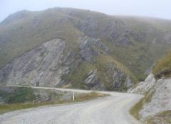
Fault Recognition 3

Back 89

1. Effects on topography or geomorphology:

- Scarps.

- Offset ridges, valleys, streams.

- Springs, sag ponds.

- Nickpoints in streams.

Front 90

Difference between slip and separation 1

Back 90

Pre-Faulting

Front 91

Difference between slip and separation 2

Back 91

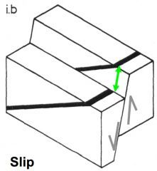
1. Slip - actual relative displacement between two points that occupied the same location before faulting.

Front 92

Difference between slip and separation 3

Back 92

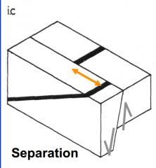
1. Separation - apparent relative displacement between two points that may have occupied the same location before faulting.

Front 93

Transposition 1

Back 93

1. Transposition occurs when a folded layer is disrupted in such a manner that the orientation of the individual segments no longer indicates the gross orientation of the parent layer.

2. There is no consistent bedding direction due to isoclinal folds.

3. Transposition structures are described from an area of semischists near Dansey Pass, North Otago, where they appear to be most strongly developed near the hinge zones of macroscopic folds. Transposition of the form surface in the hinge zone of folds in higher grade rocks is thought to be one of the reasons for the difficulty in demonstrating large folds in the Otago schists.

Front 94

Measuring X-direction of strain

Back 94

Mineral lineations: Elongate mineral grains/clasts, the long axes of the minerals are parallel to the x-axis of strain.

Front 95

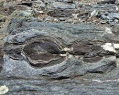
Measuring Y-direction of strain

Back 95

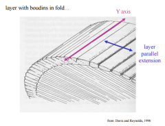
Boudins: Roughly perpendicular to the x-axis of strain, necks are parallel to y-axis.

Front 96

Measuring X-direction of strain

Back 96

The z-axis can only be measured by building a strain ellipsoid based on the from the other two directions.

Front 97

Lineations 1

Back 97

Four types: Intersection, crenulation, mineral, and linear structures.

Front 98

Lineations 2

Back 98

1. Intersection lineation: Intersection of two planar features- an "apparent" lineation in that there is no fabric that is linear.

Front 99

Lineations 3

Back 99

2. Crenulation lineation: Intersection between fold hinges and foliation.

Front 100

Lineations 4

Back 100

3. Mineral lineation: preferred alignment of minerals due to deformation and/or recrystallization during deformation.

- Stretching lineation: elongation of minerals due to "stretching" deformation and are used to infer the finite X-direction of strain.

Front 101

Lineations 5

Back 101

4. Linear structures: Boudins

Front 102

Biot's equation 1

Back 102

L = 2πt (v1/v2)^1/3 = 2πt (^3 √µ1 / 6µ2)

1. L = arc length or wavelength

2. t = strong layer thickness

3. (v1/v2) = viscosity ratio of layers

Front 103

Flinn Diagram 1

Back 103

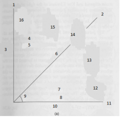
1. k = ∞

2. k = 1 or Δ (delta or change in volume) = 0

3. a = X/Y

4. Field of Constriction

5. Cigar; L-tectonite

6. Plane strain

Front 104

Flinn Diagram 2

Back 104

7. Field of Flattening

8. Hamburger; S-tectonite

9. ß

10. b = Y/Z

11. k = 0

Front 105

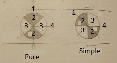
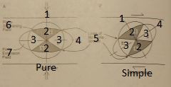
Pure Shear History

Back 105

1. Coaxial.

2. --- NFLS

Front 106

Simple Shear History

Back 106

1. Non-coaxial

2. --- NFLS

Front 107

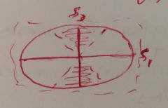
Incremental strain ellipse

Back 107

Intermediate strain steps describe separate small strain conditions; usually difficult to ascertain.

1. S3

2. S (shortening)

3. E (elongation)

4. S1

Front 108

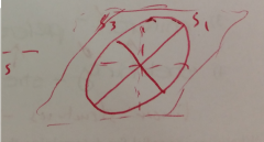
Finite strain ellipse

Back 108

Measure of the strain from an initial to final state; represents the sum of the incremental strains.

1. S3

2. S (shortening)

3. E (elongation)

4. S1

5. Lines of no finite logitudinal strain

6. Zone of Shortening

7. Zone of Elongation