![]()
![]()
![]()
Use LEFT and RIGHT arrow keys to navigate between flashcards;
Use UP and DOWN arrow keys to flip the card;
H to show hint;
A reads text to speech;
119 Cards in this Set
- Front
- Back
- 3rd side (hint)
|
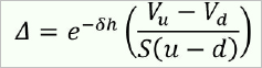
American Put Early exercise is optimal if |
PV (Interest on the strike K) > PV (Dividends) + Implicit Call By exercising a put option early - Get cash earlier, so you earn interest on K - Give up implicit call opt - Give up dividends |
|
|
|
American Call - non dividend paying stock Early exercise is optimal if |
Early exercise is never optimal. C amer = C eur Lose protection against the price of the stock going below K. Lose interest on K. |
|
|
|
American Call - dividend paying stock Early exercise is optimal if |
PV (Dividends) > PV (Interest on the strike K) + Implicit Put if early exercise is rational, exercise should be right before a div. is paid, in order to maximize the interest. |
|
|
|
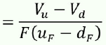
Put-Call Parity (PCP) Prepaid Forward & Forward |

|
|
|
|
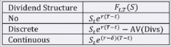
Put-Call Parity Prepaid Forward - Dividend Structure |

|
|
|
|
Put-Call Parity Forward - Dividend Structure |
|
|
|
|
PCP for Stock C - P = |

|
|
|
|
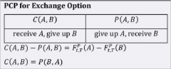
PCP for Exchange Option C(A, B) |
|
|
|
|
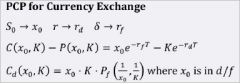
PCP for Currency Exchange S --> ? r --> ? δ --> ? |
|
|
|
|
PCP for Bonds C - P = Bt = |

|
|
|
|
Comparing Options - Different Strike Prices For K1 < K2 < K3: CALL C(K1) ? C(K2) ? C(K3) C(K1) - C(K2) ? K2 - K1 European: C(K1) - C(K2) ? PV(K2 - K1) [C(K1)-C(K2)]/[K2 - K1] ? [C(K2)-C(K3)]/[K3-K2] |

|
|
|
|
Comparing Options - Different Strike Prices For K1 < K2 < K3: Put P(K1) ? P(K2) ? P(K3) P(K1) - P(K2) ? K2 - K1 European: P(K2) - P(K1) ? PV(K2 - K1) [C(K2)-C(K1)]/[K2 - K1] ? [C(K3)-C(K2)]/[K3-K2] |

|
|
|
|
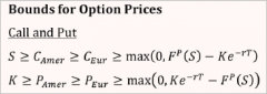
Comparing Options - Bounds for Option Prices Call and Put |
|
|
|
|
Comparing Options - Bounds for Option Prices European vs. American Call |

|
|
|
|
Comparing Options - Bounds for Option Prices European vs. American Put |

|
|
|
|
Binomial Model Replicating Portfolio |
An option can be replicated by buying delta shares of the underlying stock and lending B at the risk-free rate. |
|
|
|
Binomial Model Replicating Portfolio Delta = |
Delta - shares of underlying stock |
|
|
|
Binomial Model Replicating Portfolio B = |
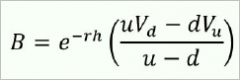
Lending B @ risk-free rate. If - then borrow to purchase stock.
|
|
|
|
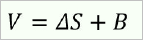
Binomial Model Replicating Portfolio V = option premium = |
|
|
|
|
Binomial Model Replicating Portfolio Table |

|
|
|
|
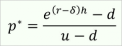
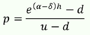
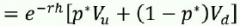
Risk-neutral Probability Pricing p* = |
|
Probability stock will increase in value. |
|
|
Risk-neutral Probability Pricing V = |
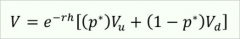
|
|
|
|
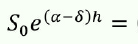
Risk-neutral Probability Pricing Se^[(r-δ)h] = |

|
|
|
|
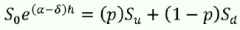
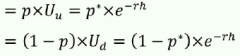
Realistic Probability Pricing p = |
|
|
|
|
Realistic Probability Pricing V = |
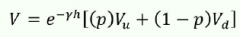
|
|
|
Realistic Probability Pricing |
|
|
|

Realistic Probability Pricing |

|
|
|
|
Standard Binomial Tree (Forward Tree) u = d = |

|
|
|
|
Binomial Model - Option on Currencies S --> ? r --> ? δ --> ? u = d = |
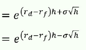
S --> x0 r --> rd δ --> rf |
|
|
|
Standard Binomial Tree (Forward Tree) p* = ... = ... |

Interestingly, r and δ don't affect p*. |
Risk neutral probability will be close to 0.5 |
|
|
Cox-Ross-Rubinstein Tree u = d = |

Centered on 1 |
If e^(r-δ) > e^σ sqrt h, violates arbitrage-free since both u & d are < e^(r-δ). With h small enough this won't happen. |
|
|
Lognormal Tree (Jarrow-Rudd Tree) u = d = |

Centered on e^(r-δ-.5σ^2)h |
|
|
|
No Arbitrage Condition |
Arbitrage is possible if the following inequality is not satisfied: d < e^[(r-δ)h] < u Means the upper node must be higher than the result of a risk-free investment and the lower node must be lower. |
|
|
|
Binomial Model - Option on Currencies S --> ? r --> ? δ --> ? p* = |
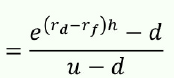
S --> x0 r --> rd δ --> rf |
|
|

Binomial Model - Option on Futures Contracts |

|
|
|
|
Binomial Model - Option on Futures Contracts T = TF = T=< St --> δ --> |
T = Expiration date of the option T = Expiration date of the futures contract T =< TF St --> Ft,TF δ --> r |
|
|
|
Binomial Model - Option on Futures Contracts p* = |
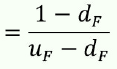
= 1/(1+u) if tree is based on forward prices
|
|
|
|
Binomial Model - Option on Futures Contracts Δ = # of forwards in replicating portfolio |
F = Futures contract price
|
|
|
|
Binomial Model - Option on Futures Contracts B = Option premium since there's no initial cost for futures |
|
|
|
|
Binomial Model - Utility Values and State Prices Options on Futures (not stocks) Uu: Ud: |
Uu: Utility value per dollar in the up state Ud: Utility value per dollar in the down state |
|
|
|
Binomial Model - Utility Values and State Prices Qu = ... = ... Qd = ... = ... |
|
|
|
|
Binomial Model - Utility Values and State Prices e^(-rh) |
= Qu + Qd |
|
|
|
Binomial Model - Utility Values and State Prices S = |
|
|
|
|
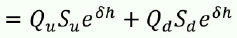
Binomial Model - Utility Values and State Prices V = |
= QuVu + QdVd |
Vd = cash flow of the stock at the EOY 1. |
|
|
Binomial Model - Utility Values and State Prices p* = |
= Qu / (Qu + Qd) |
Qi = current value of $1 paid @ EOY 1. |
|
|
ɣ |
discounting rate for option must be the same as the discounting rate for the replicating portfolio |
|
|
Binomial Model |

|
|
|
|
Futures vs. Forward Definition |
A Forward agreement is a customized contract. Futures contract is standardized / marked to market daily. Exchange traded fwd contract. |
|
|
|
The one who sells the call option is called the ... |
writer. |
|
|
|
Buy x, we are... x |
long x |
|
|
|
Sell x, we are ... x |
short x |
|
|
|
How to create a Bull Spread with Puts & Calls |
Buy K1 & sell K2. K2 > K1 |
|
|
|
How to create a Bear Spread with Puts & Calls |
Buy K2 & sell K1. K2 > K1 |
|
|
|
A Bull Spread from the perspective of the purchaser is a ... |
bear spread from the perspective of the writer. |
|
|
|
Ratio Spread |
Buy n of one option, and Sell m of another option of the same type m does not equal n |
|
|
|
Box Spread |
Agreement to buy stock @ K1 and sell it for K2. So profit = K2 - K1 (should be no gain/loss). |
|
|
|
Box Spread is a ... option strategy |
4: Bull Spread Calls & Bear Spread Puts K Bull Spread Bear Spread K1 buy call sell put K2 sell call buy put |
|
|
|
Butterfly spreads is a ... option strategy. |
3: all same type. |
|
|
|
Option prices as a function of K must be ... |
convex. |
|
|
|
Collars |
buying one option & selling an option of the othre kind. No risk. No profit or loss. |
|
|
|
Straddle |
buying 2 options of different kinds. It's a bet on volatility. (Strangle is a special subset.) |
|
|
|
Conversion |
Creating a synthetic Treasury |
|
|
|
Reverse Conversion |
Shorting stock, buy call, sell put |
|
|
|
Asset sold |
Underlying asset, St |
|
|
|
Asset want / buy |
Strike asset, Qt |
|
|
|
Foreign risk-free rate |
role of a stock to be purchased for a call option or sold for a put option. S and δ |
|
|
|
Domestic risk-free rate |
role of a cash in stock. Owner pays in a call or one which owner receives in put. The one in which the price is expressed. K |
|
|
|
Foreign Currency |
underlying asset of option |
|
|
|
TRUE / FALSE If settlement is through cash (not in currency exchange) then put options may not have the same payoff as the call option. One in f while call in domestic. Exchange rate X may be different at time t. |
TRUE |
|
|
|
A Call option cannot be worth more than ... |
underlying stock. |
|
|
|
A Euro Call cannot be worth more than ... |
prepaid forward price of the stock. If cont divs then upper bound is Se^(-δt). |
|
|
|
A Put cannot be worth more than ... |
K. |
|
|
|
A Euro Put cannot be worth more than ... |
Ke^(-rt) |
|
|
|
TRUE / FALSE An option must be worth at least zero since no negative payoff. |
TRUE |
|
|
|
A Euro option is worth at least as much as implied by ... |
Put-Call parity. |
|
|
|
For both Calls and Puts, list in order of greatest to least: S or K American option European option Max(0, Fp - Ke^(-rt)) or Max(0, Ke^(-rt) - Fp) |
S >= C amer >= C eur >= Max(0, Fp - Ke^(-rt)) K >= P amer >= P eur >= Max(0, Ke^(-rt) - Fp) |
|
|
|
TRUE / FALSE Every call option has an implicit put option built into it. Similarly, every put option has an implicit call option built into it. |
TRUE |
|
|
|
For a Euro Put option, longer time to expiry may make the PV of cash received... |
lower. |
|
|
|
A longer-lived American Call option with K increasing at the risk-free rate must be worth at least as much as a ... |
shorter-lived option. |
|
|
|
TRUE / FALSE
Longer lived American Put option is at least as valuable as the shorter-lived one, dividends or not; an increase in K is a perk. |
TRUE |
|
|
|
TRUE / FALSE An American option with expiry T and K must cast at least as much as the one with expiry t and K. |
TRUE Also true for a Euro Call option. |
|
|
|
TRUE / FALSE
A Euro Option on a nondiv paying stock with expiry T and Ke^r(T-t) must cost at least as much as one with expiry t and k. |
TRUE This statement is stronger than the previous statement & includes it. Since it applies to both calls & puts, and increases in K make calls worth less. |
|
|
|
The higher K Call |
then lower premium. The premium for a call decreases more slowly than K increases. |
|
|
|
The higher K Put |
then higher premium. The premium for a put option increases more slowly than K increases. |
|
|
|
Three inequalities - if don't hold then arbitrage |
Direction, Slope, Convexity |
|
|
|
Convexity |
Option premiums are convex. Convexity involves 3 options. |
|
|
|
Arbitrage mispricing |
If there's a mispricing, the option in the middle will be overpriced relative to other two options. So sell the middle option and buy the ones at the 2 extremes. |
|
|
|
TRUE / FALSE If a put with K1 is optimal to exercise, then so is an otherwise similar put with K=K2 > K1. |
TRUE |
|
|
|
Two ways to price options |
1. Binomial tress 2. Black Scholes |
|
|
|
Risk-Neutral assumption |
Satisfied to earn the risk-free rate on a risky asset. An option can be priced using risk-neutral prob. discounted at the risk-free rate. |
|
|
|
Law of one price |
If two portfolios lead to the same outcomes in all scenarios, they must have the same price. |
|
|
|
Risk-neutral pricing is equivalent to pricing with ... |
pricing with a replicating portfolio. |
|
|
|
B (bond) |
Amount we lend when positive. Lend @ risk-free rate. |
|
|
|
Intercept |
The intercept (the maturity value of the amt to lend) is the balancing item. |
|
|
|
Run = |
uS - dS = (u-d)S |
|
|
|
Volatility |
square root of variance
|
|
|
|
Volatility sigma_h = |
= sigma \sqrt{h} Default is annual volatility. |
|
|
|
Standard Binomial Tree Forward Tree |
Tree is based on forward prices and "the usual method in McDonald" |
|
|
|
Δ decreases to ? as the put gets further into the money. |
-1 |
|
|
|
For a call, Δ increases to ? as the call gets further into the money. |
+1 |
|
|
|
Futures contract - Early exercise |
Exercising the option enters one into a futures contract, allowing one to earn interest on the mark-to-market $. |
|
|
|
Pricing Options on Futures |
Assume Futures have the same price as Forwards. |
|
|
|
TRUE / FALSE An option may have the same expiry as the futures contract, or the futures contract may expire later. |
TRUE |
|
|
|
Futures Contract |
Pays no dividends. Almost all options on Futures are American style. |
|
|
|
Futures Contract # of shares in replicating portfolio = |
e^ (-rh) * Δ |
|
|
|
For a bond, the coupon rate serves the purpose of the ... |
dividend yield. |
|
|
|
TRUE / FALSE Bond values must converge to their maturity value, or possibly their call value if they're callable. |
TRUE |
|
|
|
Bonds are MORE/LESS volatile as period to maturity decreases. So cannot project values using fixed volatility rate. |
LESS |
|
|
|
The best way to project bond values is to project |
interest rates. |
|
|
|
Underling asset - Dividend Yield Stock/Stock Index Currency Futures Contract Bond |
Dividend Yield Dividend Yield Foreign risk free rate Risk free rate b (r) Coupon yield |
|
|
|
The discounting rate for a put option is negative since... |
you invest money at the risk-free rate & sell an asset on which you must pay a higher discounting rate. |
|
|
|
Even though the return on the underlying asset is constant, the return on the option ... |
varies by period. |
|
|
|
Price of an option computed using risk-neutral prob & discounting with r equals... |
the price using true prob. & discounting the stock with α and the option with ɣ |
|
|
|
Early exercise optimal? Higher volatility |
Less likely early exercise is optimal because of the increased value of the implicit call |
|
|
|
Random Walk |
Binomial variable in each unit of time, and as the # of periods go to infinity, the position converges to a normal dist. by CLT. |
Central Limit Theorem |
|
|
Since we're multiplying rather than adding moves to model stock prices .. |
the stock price converges to the exponential of a normal dist. or a lognormal dist. |
|
|
|
Lognormal Model for Stock prices Assumptions |
1. Volatility is constant 2. Stock returns for diff. time periods are indep. 3. Large stock movements do not occur; stock prices do not jump. |
All of these assumptions appear to be violated in practice. |
|
|
Cox-Ross-Rubinstein tree & Lognormal tree |
Do not guarantee arbitrage-free. Upper node > forward price Lower node < forward price |
|
|
|
Binomial model For an infinitely lived Call option on a stock with σ = 0, |
exercise is optimal if Sδ > Kr |
|