Quantitative Economics

Front 1

What is the Conditional Expectations Function?

Back 1

The CEF of a variable Yi given a covariate Xi is the expectation, or population average, of Yi with Xi held fixed

It is written as E[Yᵢ|Xᵢ] and is regarded as a function of Xᵢ. So it shows you how the mean of something changes as you change something else.

It can also be written as Yᵢ = E[Yᵢ|Xᵢ] + eᵢ

Change the Value of Xᵢ, to trace out the CEF

For a particular value of Xᵢ, say x, the notation is:

E[Yᵢ|Xᵢ = x]. The function does not have to be linear.

Front 2

CEF Decomposition: What can the variable Yᵢ be broken up into?

What does this intuitively mean?

Back 2

1. The CEF

- A description of how, on average, it varies with some other variable Xᵢ

- This is the bit which is explained by Xᵢ

2. A Residual:

- This is orthogonal to Xᵢ (i.e. uncorrelated with Xᵢ)

- This is the bit which isn't explained by Xᵢ

Front 3

What are the special properties of the residual term in the CEF decomposition?

Back 3

- It is mean independent of Xᵢ, i.e. E[eᵢ|xᵢ] = 0.... - this itself follows from Law of Iterated Expectations (proven by rearranging the CEF decomposition in terms of the residual)

- It is uncorrelated with any function of Xᵢ... also uses LIE to prove that E[h(xᵢ).eᵢ] =0

Front 4

Prove mean independence of the residual term in the CEF decomposition of Yᵢ.

What is the result you should end up with?

Back 4

- Rearrange the CEF decomposition in terms of the residual.

- Take expectations given Xᵢ.

- Use the Law of Iterated Expectations

- End up with E[eᵢ|xᵢ] = 0

Front 5

Prove uncorrelatedness (of the residual term in the CEF decomposition) with Xᵢ or any function of Xᵢ.

What is the result you should end up with?

Back 5

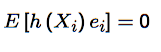
Take a function of the variable Xᵢ, i.e. h(Xᵢ)

- Multiply it by the residual: h(Xᵢ) eᵢ

- Take expectations: E[h(Xᵢ) eᵢ]

- Use the law of iterated expectations, i.e. take expectations of all of the above given Xᵢ

- Then note that we are taking expectations holding Xᵢ fixed, so h(Xᵢ) is also fixed and can be taken out of the inner expectation function

- By mean independence, the remaining term inside the inner expectation is zero

- We therefore end up with the result at the top

Front 6

The CEF Decomposition of Variance:

Decompose the variance of Yᵢ involving the CEF.

What are the two bits it is decomposed into?

Back 6

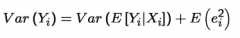
Use the equation: Yᵢ = E[Yᵢ|Xᵢ] + eᵢ

- Take Variances of both sides

- The covariance term on the RHS that emerges will collapse to zero, since eᵢ is uncorrelated with any function of Xᵢ

- Then for the error term, use the definition of variance to decompose it into two, the Law of Iterated Expectations and mean independence to collapse one of these two to zero

- End up with equation above

Decomposed into:

1. The Variance of the CEF

2. The Variance of the Residual

Front 7

When considering the CEF as a predictor, what is:

- A best predictor of Yᵢ?

- A loss function?

Back 7

Presuming that we observe some variable Xᵢ and wish to predict some other variable Yᵢ.

Let m(Xᵢ) denote a predictor of Yᵢ which uses Xᵢ

- A best predictor of Yᵢ conditional on Xᵢ is a prediction that minimises the expected loss with respect to a specified loss function

- A loss function can be thought of as a function which penalises predictions which are inaccurate

Front 8

What does the loss function actually measure (mathematically/notationally)?

Back 8

A measure of inaccuracy is the size of the deviation between Yᵢ and the prediction m(Xᵢ):

eᵢ = Yᵢ - m(Xᵢ)

A loss function L(eᵢ) is a function of eᵢ which penalises inaccuracy.

L has the property that bigger eᵢ's in either direction (i.e. worse predictions) means a bigger loss (this is normally symmetric either side, but its up to you).

Front 9

What is the conditional prediction problem?

Back 9

Given a chosen L (i.e. that describes the loss function L(eᵢ)), the conditional prediction problem is to select the predictor m(Xᵢ) (where eᵢ = Yᵢ - m(Xᵢ) ) which minimises the expected value of the loss function (i.e. minimises the expected inaccuracy of the prediction).

Choose m(Xᵢ) to minimise E[L(eᵢ)]

i.e. choose the function m(Xᵢ) to minimise the expected loss when m(Xᵢ) is used to predict Yᵢ.

Front 10

As a loss function, what is the "squared loss", or "squared error"?

What properties does it have?

Back 10

The squared error is a measure of the squared "distance" between Yᵢ and m(Xᵢ).

- L(eᵢ) = eᵢ² = [Yᵢ - m(Xᵢ)]²

This interpretation remains even when we move to the expected loss:

- E[L(eᵢ)] = E[eᵢ²]

- This loss function penalises bigger prediction errors by more than smaller prediction errors

- It assigns no loss to predictions which are bang on, i.e. L(0) = 0

- It penalises bad predictions symmetrically (regardless of the sign of the error), i.e. L(eᵢ) = L(-eᵢ)

Front 11

To what is the CEF the solution?

Write this in notation.

Back 11

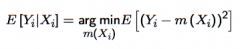
The CEF is the solution to a conditional prediction problem when L is the squared loss.

The equation tells us which predictor is the best one given this notion of "bestness" (i.e. reducing the squared loss).

The CEF is the argument which minimises the expected loss, where the loss is the "squared loss" loss function.

So, setting the argument m(Xᵢ) = E[Yᵢ|Xᵢ] minimises the expected loss

Front 12

Show that the CEF is the best predictor of Yᵢ in the least squares sense.

(i.e. solve the Conditional prediction problem when L is the "squared loss" loss function).

What do you want to end up with?

Back 12

You will eventually want to take the expectation of the square of the residual

- so start with the residual and square it: [Yᵢ - m(Xᵢ)]²

- Add and subtract E[Yᵢ|Xᵢ], i.e. the CEF, within the squared term

- Expand out the quadratic to get three terms

You need to minimise this big expression's expectation by choosing m(Xᵢ)

- The first term doesn't involve m(Xᵢ) so you can disregard it

- The second term contains Yᵢ - E[Yᵢ|Xᵢ], i.e. the error term, and a function of Xᵢ. But by uncorrelatedness, this is zero too, so you can disregard it.

- The final term is a simple quadratic:

(E[Yᵢ|Xᵢ] - m(Xᵢ))². This is just minimised (at zero) where E[Yᵢ|Xᵢ] = m(Xᵢ)

- This helps you end up with the equation (solution) at the top.

Front 13

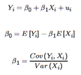
What is the Linear Regression Model?

Write it in notation.

What is it simply/intuitively?

Back 13

The Linear Regression model is a linear model of the CEF.

In notation: E[Yᵢ|Xᵢ]≅b₀+b₁Xᵢ

Intuitively, it is just a simplified description/idealisation of the CEF.

NOTE: Parameters: b₀, b₁ in this case (or regression residuals). Anything part of a regression that is not data is a parameter.

Front 14

Is the Linear Regression the same as the CEF?

What does this imply for the residuals from the regression and from the CEF decomposition?

Back 14

The Linear Regression model is just a linear model of the CEF.

- Intuitively, it is just a simplified description/idealisation of the CEF.

Unless the CEF really is linear, then the CEF and the linear regression are not the same.

This means that the residuals from the regression (uᵢ) are not the same as the residuals from the CEF decomposition (eᵢ).

- Yᵢ = E[Yᵢ|Xᵢ] + eᵢ

- Yᵢ = [b₀+b₁Xᵢ] + uᵢ

Front 15

What is "computing the linear regression"?

(Notationally, e.g. finding what values)

Back 15

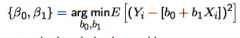
Given the linear regression model: Yᵢ = [b₀+b₁Xᵢ] + uᵢ

- Computing the linear regression model just means finding the values of {b₀, b₁} which minimise the expected loss (the expected sum of squares)

- The optimal values are denoted by {β₀, β₁}

- These values satisfy the equation (containing the argument) above

Front 16

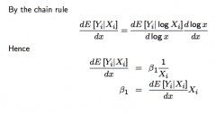
Mechanically, compute the linear regression.

Back 16

You must solve the optimisation problem:

Find {β₀, β₁} as the optimal argument of {b,₀ b₁} that solves: min E[(Y-[b₀+b₁Xᵢ])²]

First, take FOC w.r.t. b₀ and set it equal to zero

- You end up with E[Yᵢ - b₀ - b₁Xᵢ] = 0, i.e. E[uᵢ] = 0, i.e. the optimal values are such that the residual error is zero on average

Second, take FOC w.r.t. b₁ and set it equal to zero.

- You end up with E[(Yᵢ - b₀ - b₁Xᵢ).Xᵢ] = 0, i.e. E[uᵢ.Xᵢ] = 0, i.e. the optimal values are such that the residual is uncorrelated with Xᵢ (This follows itself just from the definitions of correlation, and covariance, etc.)

Then use these conditions as simultaneous equations, to solve for the optimal {β₀, β₁}

- Substitute the first into the second to obtain β₁

- Then sub β₁ in to find β₀

End up with values for β a₀nd β₁ at the top.

- These are just the intercept and gradient terms of the Linear Regression Model

Front 17

What is the justification for using linear regression?

Back 17

1. It is the best linear predictor of Yᵢ (less important) - in the least squares sense, that is.

- This is by proof of computing the linear regression parameters, since we minimise the expected squared loss.

2. It is the best linear approximation to the CEF (more important).

- This means that it is more simple and straightforward to deal with than the CEF.

- This is proven by showing that the values of {b, ₀b₁} that solve the CEF approximation problem (i.e. minimise the expectation of the squared distance between the (maybe wiggly) CEF and a linear function of Xᵢ) are the same values that solve the the linear least squares problem.

Front 18

Prove that the Linear Regression is the best linear approximation to the CEF

... i.e. prove that the regression parameters you obtain by computing the linear regression (solving the linear least squares problem) ALSO solve the CEF approximation problem

Back 18

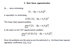
This is proven by showing that the values of {b, ₀b₁} that solve the CEF approximation problem (i.e. minimise the expectation of the squared distance between the (maybe wiggly) CEF and a linear function of Xᵢ) are the same values that solve the the linear least squares problem.

To do this:

- Focus on the minimand in the latter problem above

- Add and subtract the CEF within the squared term (i.e. to "get it involved" since we want to end up with a term involving it!)

- Expand out the brackets and get three terms

- The first is irrelevant and doesn't contain b₀ or b₁

- The second term by uncorrelatedness is zero.

- The third term is what's left, and this was the minimand in the FIRST minimisation problem

- Since the problems are the same, so are the solutions!

- Now look at the slide (above) for the rest of the proof!

Front 19

Explain how to extend the bivariate regression to multiple regression, i.e. state the formulae for the intercept and each coefficient.

Include the Frisch-Waugh-Lovell Theorem and it's intuition

Back 19

For the intcerept:

- In the Bivariate case: β₀ = E[Yᵢ] - β₁E[Xᵢ]

- In the multivariate case: β₀ = E[Yᵢ] - β₁E[X₁ᵢ] - β₂E[X₂ᵢ] - ... - βKE[XKᵢ]

For the coefficient term:

- In the Bivariate case: β₁ = Cov(Yᵢ, Xᵢ) / Var(Xᵢ)

- In the multivariate case: βk = Cov(Yᵢ, X˜kᵢ) / Var(X˜kᵢ)

- This result is the Frisch-Waugh-Lovell Theorem

Intuition:

- X˜kᵢ is the residual term from a regression of Xkᵢ on all of the other regressors (i.e. X₁ᵢ to Xkᵢ excluding Xkᵢ)

- X˜kᵢ can thus be thought of as the variation in Xkᵢ which cannot be explained by all other regressors

- The bivariate regression of Yᵢ on X˜kᵢ therefore focuses on the problem of predicting Yᵢ using just the independent variation in Xkᵢ with the effects of the other regressors removed.

- i.e... The coefficient βk on Xkᵢ can be thought of as a simple bivariate regression of Yᵢ on Xkᵢ once you have dealt with all the other regressors.

Extending this idea to the rest of the regressors, means that the coefficients all reflect the predictive contribution of each regressor alone.

Front 20

What is (multi)collinearity in a multivariate regression?

What does this imply for the residual from the regression of one variable on all other variables in the multivariate regression?

What does this imply for the coefficient of this variable in the multivariate regression?

What does perfect multicollinearity imply for computing the OLS estimator?

Back 20

(Multi)collinearity is when Xkᵢ is perfectly explained by the other regressors.

- Xᵢ is a (perfect) linear function of the other regressors

This implies that the residual from the regression of Xkᵢ on all other variables in a multivariate regression is zero, i.e. X˜kᵢ = 0.

Under perfect multicollinearity, it is not possible yo compete the OLS estimator.

This implies that it has no independent contribution to the prediction problem, and the coefficient is therefore also zero, i.e. βk = 0.

Front 21

How is the conditional expectation/conditional mean theoretically calculated.

In practice, how could it be calculated?

Back 21

In Theory:

- Using our linear model describing the CEF:

E [Yᵢ|X₁ᵢ, X₂ᵢ] = β₀+ β₁X₁ᵢ + β₂X₂ᵢ

- We can use particular values of the covariates X₁ᵢ = x₁, and X₂ᵢ = x₂ to give the conditional mean: E [Yᵢ|X₁ᵢ = x₁, X₂ᵢ = x₂] = β₀+ β₁x₁ + β₂x₂

In Practice:

- We could slice all our data by by hand, and look at individual cells, i.e. looking for values of Yᵢ whenever X₁ᵢ = x₁ and X₂ᵢ = x₂.

- Run a regression, which interpolates/extrapolates and "fills in" any empty cells (i.e. where there are no observations conditional on the values of the covariates).

.... Regression is only approximate, but much more efficient. Also, it is still the "best approximation" in the least squares sense.

Front 22

What is the interpretation of the intercept in a linear regression?

Back 22

The interpretation of the intercept is as a prediction when all the covariates are 0.

This is the conditional expectation of Yᵢ if everything else is zero.

This "condition" may never even happen in the data, but the regression allows you to extrapolate.

Front 23

What are the two possible interpretations of the "slope" coefficients in a linear regression?

Are they always useful/appropriate?

Back 23

1. Literal/Descriptive Interpretation

- This follows directly from the Frisch-Waugh-Lovel theorem: the coefficients are the measures of the partial correlation between Yᵢ and each explanatory variable, netting out the effect of the other variables

- This measures the degree of linear association between Yᵢ and the residual variation in each explanatory variable independently

- This interpretation is purely descriptive, always useful and always appropriate

2. Causal Interpretation

- That they measure the effect of ceteris paribus exogenous changes in each explanatory variable on the dependent variable Yᵢ

- This interpretation is causal, extremely important (but if and only if its warranted), and may be completely wrong.

Front 24

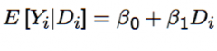
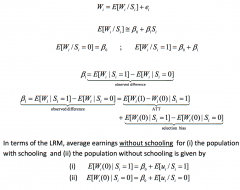
When does the coefficient β₁ in this linear regression support a descriptive interpretation. and, when does it support a causal interpretation?

Back 24

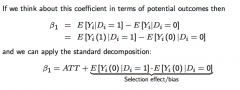
β₁ is the computed difference in conditional expectations for Dᵢ = 0 and Dᵢ = 1 in this linear regression.

In terms of the potential outcomes framework, this contains the ATT plus Selection Bias.

1. The coefficient always supports a descriptive interpretation as the difference between average observed outcomes between the Dᵢ = 1 group and Dᵢ = 0 group.

2. The coefficient only supports the interpretation of the casual effect of Dᵢ on Yᵢ if selection bias is absent (i.e. only if Dᵢ is independent of potential outcomes Yᵢ).

Front 25

How is the Conditional Independence Assumption relevant to Linear Regression?

Back 25

Using multiple regression combined with the Conditional Independence Assumption (CIA) legitimises the interpretation of slope coefficients as. causal effects.

The idea is to add relevant regressors until all of the systematic (non-random) variation in Dᵢ has been accounted for, so that, conditional on these covariates, Dᵢ is independent of potential outcomes.

.... i.e. adding multiple regressors until you have "soaked up" all the non-randomisation

Adding regressors often increases the credibility of the causal interpretation as long as those new regressors do not themselves introduce selection bias.

Under the CIA, Dᵢ is independent of {Yᵢ(0), Yᵢ(1)}|Xᵢ and so the means/expected outcomes for both groups Dᵢ = 0 and Dᵢ = 1 are the same (conditional on Xᵢ = x).

Front 26

Why would the causal interpretation of β₁ hold for any value of Xᵢ in a linear regression with the conditional independence assumption implied.

Back 26

The regression model is linear, so whatever value Xᵢ, the causal effect of Dᵢ conditional on Xᵢ will always be β₁.

So β₁ = ATT|Xᵢ = x,

= the unconditional ATT

= the ATE

Front 27

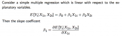
...measures what?

Differentiate between the explanatory variable being continuous, binary, and ordered-discrete

Back 27

Assuming it's causal causal (i.e. no selection bias), then this measures the effect of:

- (If continuous) a small exogenous change in X₁ᵢ on the dependent variable, or the "marginal effect of" X₁ᵢ on Yᵢ

- (if binary) being in the X₁ᵢ = 1 group versus the X₁ᵢ = 0 group, i.e. written with Δ instead of ∂

... but this is basically still an approximate partial derivative

- (if ordered-discrete), then β₁ᵢ is the effect of a one unit-increase in X₁ᵢ

Front 28

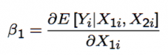
If a regression has higher-order terms, then what is the marginal effect of each variable a function of?

Differentiate between the explanatory variable being continuous, binary, and ordered-discrete

Back 28

- Continuous: The marginal effect of the variable is a function of the level of that variable.

- Binary: higher order terms do not arise

- Ordered-discrete: We reply on the continuos interpretation described above, but acknowledge that this is an approximation.

... the quality of this approximation depends on the size of the "steps" in X₂ᵢ

Front 29

That the marginal effect of one variable may depend on the value of another variable is symptomatic of what kind of terms in the regression?

Back 29

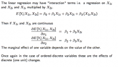
Answer: Interaction Terms.

Example: If there is an interaction term, then "returns to education may depend on the colour of your skin."

Front 30

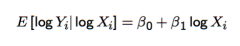
If we are working with the natural log of the dependent variable Yᵢ, and model the CEF as:

E[log Yᵢ|X₁ᵢ] = β₀ + β₁X₁ᵢ

...Then (use Jensen's Inequality to) approximate the CEF in terms of e.

Back 30

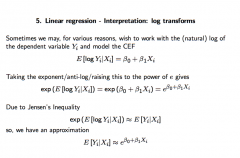
(Joe: You can basically forget the Jensen's inequality thing, and just take expectation to cancel out the log on the LHS).

Final result above.

Front 31

What does differentiating the log-transformed CEF approximation (i.e. where the dependent variable is log transformed) and rearranging for β₁ give?

... i.e. What does β₁ represent notationally?

When substituting in for the definition of CEF elasticity (i.e. (proportional effect on E[Yᵢ|Xᵢ]) / (proportional change in Xᵢ), what does this give us intuitively?

Back 31

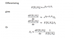
Differentiating this gives β₁ ≅ ε / Xᵢ

... where ε is the elasticity of the conditional expectation E[Yᵢ|Xᵢ] w.r.t. the explanatory variable.

Intuitively:

β₁ ≅ (the proportional effect on E[Yᵢ|Xᵢ] ) / (The change in Xᵢ)

... so β₁ captures the proportional effect on the expected value of Yᵢ of a marginal change in Xᵢ,

...e.g. a one unit increase in Xᵢ changes E[Yᵢ|Xᵢ] by (β₁ x 100) percent (approximately)

Front 32

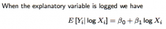
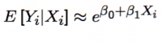
What does differentiating the CEF approximation (i.e. where the explanatory variable is log transformed) and rearranging for β₁ give?

Back 32

Differentiating this gives β₁ ≅ ε.E[Yᵢ|Xᵢ]

... where ε is the elasticity of the conditional expectation E[Yᵢ|Xᵢ] w.r.t. the explanatory variable.

Intuitively:

β₁ ≅ (the effect on E[Yᵢ|Xᵢ] ) / (The proportional change in Xᵢ)... so β₁ captures the effect on the expected value of Yᵢ of a small proportional change in Xᵢ.

... e.g. a one percent increase in Xᵢ changes E[Yᵢ|Xᵢ] by (β₁/100) percent (approximately)

Front 33

What does differentiating the CEF approximation (i.e. where both the explanatory variable and the dependent variable is log transformed) and rearranging for β₁ give?

... i.e. What does β₁ represent notationally?

When substituting in for the definition of elasticity, (i.e. (proportional effect on E[Yᵢ|Xᵢ]) / (proportional change in Xᵢ) what does this give us intuitively?

Back 33

Differentiating this gives β₁ ≅ ε

... where ε is the elasticity of the conditional expectation E[Yᵢ|Xᵢ] w.r.t. the explanatory variable.

Intuitively:

- β₁ is just (approximately) the definition of elasticity of the expected value of Yᵢ w.r.t. Xᵢ

- β₁ ≅ (the proportional change in E[Yᵢ|Xᵢ] ) / (The proportional change in Xᵢ)

... e.g. a one percent increase in Xᵢ changes E[Yᵢ|Xᵢ] by β₁ percent (approximately)

Front 34

What is the difference between Cross-section data, Time-series data, and Panel data?

Back 34

Cross Section: Data on different entities (e.g. workers, consumers, firms, etc.) for a single time period

Time-Series: Data for a single entity (e.g. a person, firm, or country) relating to multiple time periods

Panel: Data for multiple entities in which each entity is observed at two or more time periods

Front 35

What is Simple Random Sampling?

What does it mean to be identically and independently distributed?

Back 35

- n objects selected at random from a population

- each member of the population is equally likely to be included in the sample

Identically Distributed: Randomly drawn from the same population

Independently Distributed: (Random Sampling implies that) knowing the value of Y₁ provides no information about the value for Y₂

Front 36

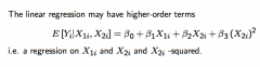
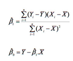
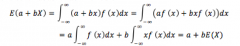
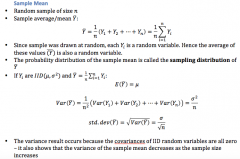
What is the distribution (i.e. mean and variance) of the sample mean Ȳ, when the sample is IID, and the population has mean µ and variance σ²?

Back 36

E[Ȳ] = µ

Var(Ȳ) = σ²/n

To find these, define Ȳ as (1/n)(Y₁+Y₂+...Yn)

Front 37

What are the exact and approximate/asymptotic approaches to sampling distribution?

What are the two key tools to approximate sampling distributions?

Back 37

Exact: exact distribution or finite same distribution, holds exactly for any n

- If Yᵢ ~ N(µ,σ²) and a sample from it is IID then its sample mean Ȳ ~ N(µ,σ²/n)

- If Y is not normal, then deriving the exact sampling distribution is complicated

Approximate: approximations to the sampling distribution that rely on n being large. Approximations became exacts as n → ∞

Two key tools to approximate sampling distributions:

- Law of Large Numbers: If sample is IID, and variance σ² is finite, then the sample mean will be near µ with increasing probability as n increases, i.e. convergence in probability, or consistency

- Central Limit Theorem: If sample is IID, then under general conditions, the distribution of the sample mean is well approximated by a normal distribution when n is large

Front 38

What are the OLS estimators?

Back 38

Ordinary Least Squares Estimators are the sample equivalents of the parameters of the liner regression model, i.e. using X̄ and Ȳ instead of E[X] and E[Y] to find the above.

Front 39

What are the properties of the OLS estimators β₁ˆ, β₂ˆ, under a general set of assumptions?

What are those assumptions?

Back 39

Properties:

- They are unbiased estimators of the population parameters

- Among the set of linear unbiased estimators, the OLS estimators have the smallest variances

- They are the Best Linear Unbiased Estimators (BLUE)

- If the sample size if sufficiently large (then by the CLT), the OLS estimator is well approximated by the bivariate normal distribution. Their marginal distribution are normal in large samples

- If the sample size is large (then by the LLN), the OLS estimators will be close to the true population values with high probability, i.e. consistency

Assumptions:

- Conditional Distribution of the error term uᵢ given Xᵢ has a mean of zero, i.e. mean independence, i.e. your error term captures only random things and everything that systematically affects Y is already captured in your model - this assumption is critical if the OLS estimator is to have "good" properties

- Samples of Xᵢ and Yᵢ are IID

Front 40

Why is the variance of β₁ˆ inversely related to the variance in X, i.e. the data?

Back 40

More variance in X means that there is more variation in the data that can be used to estimate the regression line.

Front 41

What is the regression R²?

Back 41

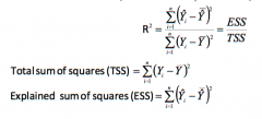
The regression R² is a measure of how well the OLS regression line fits the data. It is essentially the fraction of variance in the sample that is explained by the regression.

It is the fraction of sample variance of Yᵢ explained by the OLS regression and ranges between 0 and 1 in value.

R² is the ratio of the sample variance of Yᵢˆ to the sample variance of Yᵢ

It can also be defined in terms of what the regression can't explain (i.e. the Sum of Squared Residuals)

R² = ESS/TSS = 1 - SSR/TSS

Front 42

What is the Standard Error of the Regression (SER) and how do you calculate it?

Does this change if we are conducting a multiple regression?

Back 42

The Standard Error of the Regression (SER) is an estimator of the standard deviation of the regression term uᵢ. Like the Regression R², it is another measure of goodness of fit.

SER = √[ SSR/(n-2) ]

We divide by n - 2, since SSR (and therefore SER) is computed using two OLS residuals (i.e. we are estimating the slope parameter and the constant term).

In a multiple regression, SER = √[ SSR/(n - k -1) ]

since we are estimating k+1 parameters from the sample (i.e. k regressors plus the intercept).

Front 43

What is the adjusted R² and why is it important?

Back 43

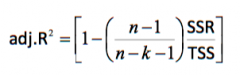
Introducing an additional regressor into the regression mode invariably reduces the SSR (or increases the ESS) and hence increases the R² even if the regressor has negligible explanatory power.

But adding addition regressors means estimating more parameters from a given sample, and so reduces the degrees of freedom and increases the SER.

Therefore, the adjust R² corrects this problem by penalising you for including another regressor - this does not always increase when you add another regressor.

Front 44

Why can't we test coefficients "one at a time" as a proxy for testing a joint hypothesis about regression parameters?

What is a more efficient way (other than just correcting the one-at-a-time approach to the significance level for the joint test is correct) to take into account the joint distribution of the estimators?

Back 44

Using the individual t-statsitcs from testing the parameters one at a time as a proxy for testing the joint null hypothesis distorts that size of the joint test (i.e. the actual rejection rate under the null)

Intuitively:

We could reject the joint hypothesis if:

- One is non-zero

- The other is non-zero

- Or both are non-zero

"one-at-a-time" tests does not capture this final possibility, so doing so would be using a distorted significance level.

The more efficient way is to use an F-test.

Front 45

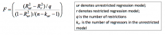
How would you conduct an F-test?

What is the F-statistic and what does it really measure?

Back 45

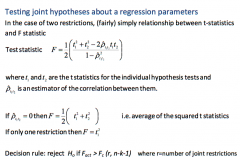
The F-statistic takes into account the joint distribution of the estimators.

Front 46

What is the "Rule of Thumb" F-statistic ?

What is the intuition behind it?

How/when can it be used?

Back 46

Intuition:

- If certain explanatory variables (e.g. X and Y) are important determinants of the dependent variable, then including them in a regression should substantially improve the fit of the regression

- A large value in the R² when these variable are included should be associated with a large value of the F-statistic for the hypothesis H₀: βᵪ = βᵧ = 0

How/when should it be used?

- Only applies exactly under additional assumptions about the variance of the errors uᵢ (i.e. homoscedasticity, where variance is constant for all i)

- More generally, the relationship is not exact, and it should only be used as a diagnostic

Front 47

What is the dummy variable trap?

Back 47

The Dummy Variable trap is a scenario in which the independent variables are multi collinear

- one variable can be predicted from the others

- e.g. including both a 'white' and 'non-white' regressor.

- They will always sum to one, and so can be predicted by each other

- One of these variables is redundant - it has no new information to add

Front 48

What is imperfect multicollinearity?

What are its consequences for OLS estimator variance and confidence intervals?

What is the intuition behind why it is a problem?

Back 48

Two of more regressors are highly correlated (but not perfectly correlated), and so cannot be perfectly derived as a linear combination of the others.

- One or more of the coefficients will be imprecisely estimated

Consequences:

- The variance of the OLS estimator of the coefficient on variable 2 will be large

- Confidence Intervals for this coefficient will be wide

- Essentially, the OLS estimator is just less precise, since the OLS estimator itself treats to identify a marginal effect with a ceteris paribus assumption (a condition which a high correlation would violate)

Intuition:

- The coefficient on variable 1 is the fact on of variable 1 on Y independent of variable 2

- but if variable 1 and variable 2 are highly correlated in the sample, then there is very little variation in variable 1 that is independent of variation in variable 2 (i.e. if we were to hold variable 2 constant)

- There are large standard errors for the OLS coefficients, so we have smaller t-statistics and more likely to not reject H₀

- The data are therefore pretty much uninformative about what happens to Y when variable 1 changes but variable 2 doesn't?

Front 49

What assumption plays a key role in establishing the properties of the OLS estimator?

Which properties are these?

Back 49

The Mean independence assumption, i.e. E[u|xᵢ] = 0

If E[u|xᵢ] = 0, then it follows that:

- E[uᵢ] = 0

- Cov(Xᵢ, uᵢ) = 0

This helps to establish properties of the OLS estimator:

- Unbiasedness

- Consistency

- Large sample normal distribution of the estimator

Front 50

What is a causal relationship?

Back 50

A causal relationship (e.g. between schooling and earnings) is the functional relationship describing what a given individual wold earn if she obtained different levels of education:

- It tells us what individuals earn on average if we could either change their schooling holding everything else fixed

- Or it tell us what individuals earn on average if we could change their schooling randomly, i.e. if schooling were randomly assigned

Front 51

When is β₁ in the linear regression model a causal effect, i.e. when does it have a causal interpretation?

What is the name of this causal effect?

Show why the mean independence assumption is important to conclude that there is no selection bias.

Back 51

The conditional independence assumption (in the context of the leaner regression model, i.e. E[uᵢ|X] = 0) must hold for the coefficients of the linear regression model to have a causal interpretation.

If Sᵢ (the treatment variable) is independent of potential outcomes, then selection basis zero and the regression coefficient β₁ has a causal interpretation.

β₁ = average treatment effect for the treated (ATT)

This formal selection bias term contains error terms.

- So If E[u|Sᵢ] = 0, then there is no selection bias.

Front 52

How can we extend the CEF to mitigate selection bias?

Then what would β₁ in the linear regression model measure?

Does it measure the ATT?

Back 52

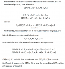
We can extend the CEF to condition on a characteristic that somehow causes the two treatment groups to be different.

- define that variable Xᵢ = 1 or Xᵢ = 0

Now β₁ measures the difference in observed outcomes for group Xᵢ = x

If there is no remaining selection bias, i.e. E[vᵢ|Sᵢ, Xᵢ] = 0, i.e. new residual term now is mean independent (conditional on Xᵢ and Sᵢ), (i.e. the Conditional Independence Assumption), then β₁ measures the ATT for Xᵢ = x (and the unconditional ATT and ATE because o linearity..?)

Front 53

Given a correctly specified model, what is the implication for the error term and hence the OLS estimator in an estimated model if we omitted a variable?

When is the OLS coefficient in the estimated model an unbiased estimator of the OLS coefficient in the correctly specified model?

- does it matter whether the underlying CEF is linear?

- If so, what would this problem be called?

Back 53

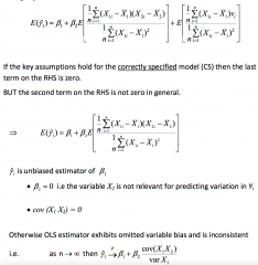
Correctly-specified ("true"-ish) model:

- Yᵢ = β₀+βᵢX₁ᵢ+β₂X₂ᵢ + vᵢ

- Well-specified: good approximation to CEF and error term satisfies the conditional mean zero assumption

The estimated model omits X₂ (may be unobservable or it is innately difficult to measure)

- Yᵢ = γ₀+γ₁X₁ᵢ + uᵢ

- The error term uᵢ will be a composite of omitted variable X₂ᵢ and the error term of the correctly-specified linear model vᵢ

- So E[uᵢ|X|] ≠ 0

We can then also prove that E[γ₁] = β₁ + (some other stuff as a function of β₂)

➡ it will in general be a biased estimator (even if the key assumptions hold for the correctly specified model)

Assuming that those key assumptions do hold... γ₁ will only be an unbiased estimator if:

- β₂=, i.e. the variable X₂ is not relevant for predicting variation in Yᵢ

- Cov (X₁, X₂) = 0, i.e. covariance between included and omitted variable is zero - if they are uncorrelated in the population, then there is no bias, or if there is no systematic relationship between them

Otherwise, the OLS estimator exhibits omitted variable bias and is inconsistent.

- even when n is large, it is still inconsistent...

The OLS estimator is also biased and inconsistent, i.r. the underlying CEF (that the linear regression is attempting to approximate) is non-linear:

- If E[Yᵢ|Xᵢ] = h(Xᵢ) where h(.) is a function that can be well-approximate by a polynomial of some high degree

- then when we approximate the CEF by the simple linear regression model, we will end up omitting important higher-order terms that describe the CEF

- So again, E[uᵢ|Xᵢ]=0

- This is misspecification of function form

Front 54

What is the tradeoff between omitted variable bias and variance?

Back 54

Leaving out relevant variables introduces bias.

But throwing everything in (if in doubt over its relevance) also has costs.

Including a variable that is not relevant to predicting Yᵢ:

- increases the standard errors (estimators of standard deviation) of the other regression parameters

- it reduces the degrees of freedom and hence increases the Standard Error of Regression (SER) as well as increasing R² etc.

Front 55

What is a Bad control in a regression?

Why is this a problem?

Back 55

A bad control is a variable that is itself an outcome variable for the "experiment" at hand

A good control is a variable that can be thought of as having been fixed at the time the regressor of interest was determined.

This leads to selection bias, since:

- E[uᵢ|Xᵢᵇᵃᵈ =0]

Front 56

What is simultaneous causality?

Give an example.

Back 56

Simultaneous Causality:

- Generally, the underlying idea of regression is that by including the value of Xkᵢ in a liner regression model, we are better able to produce the value of Yᵢ

- But SC is when the reverse is (also) true, i.e. by using the value of Yᵢ in a linear regression model, we are better able to predict the value of Xkᵢ

Example: Regression test scores on Student-teacher ratios

- but suppose government provides additional funding for teachers in areas with low average test score

- If other variables explain the variation in STR, then the error term in the original regression of test scores on S-T ratios will not be mean independent, i.e. E[uᵢ|STRᵢ] ≠ 0

Front 57

Why are measurement errors (errors-in-variables) a problem in a linear regression model?

Back 57

Suppose there is a correctly/well-specified model:

Yᵢ = β₀+ β₁Xᵢ* + vᵢ

-so it is a good approximation to the CEF

- the error term vᵢ satisfies the assumption of zero conditional mean

If we estimated it correctly

- the regression coefficients have causal interpretation

- the OLS estimates of regression coefficients are unbiased etc.

But suppose we only observe Xᵢ* with error, i.e. we actually only observe Xᵢ such that

Xᵢ = Xᵢ* + 𝛆ᵢ

In our estimated model, the residual term uᵢ is a composite of:

- the error term in the correctly specified model

- and the measurement error 𝛆ᵢ

Xᵢ and 𝛆ᵢ are correlated ➡ Xᵢ and uᵢ are correlated ➡ E[uᵢ|Xᵢ] ≠ 0

Front 58

What do measurement errors imply for the bias of the OLS estimator?

What is this bias referred to as? Why?

What does this mean intuitively?

Back 58

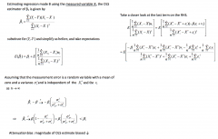
If we estimate a regression (Yᵢ = β₀ +β₁Xᵢ + uᵢ) using the measured variable Xᵢ, where Xᵢ = Xᵢ* + 𝛆ᵢ, and the true variable is Xᵢ = Xᵢ* + 𝛆ᵢ

- start with the equation for β₁ˆ

- substitute in the standard (Y- Y¯) linear regression equation in for (Y - Y¯) in the equation

- Simplify, then take expectations

- Sub in for Xᵢ = Xᵢ* + 𝛆ᵢ, and uᵢ = -β𝛆ᵢ + vᵢ, where vᵢ was the error term in the correctly specified model

- Then multiply out and simplify

- We end up β₁ˆ →ⁿ β₁(σ²𝑥/(σ²𝑥+ σ²𝜺)) < β₁

- So the OLS estimator is biased downwards (in absolute magnitude)

This is therefore referred to as attenuation bias.

This means that we tend to underestimate causal effects if we measure a variable with error.

Front 59

What is regression pathology concerned with?

What are 4 sets of circumstances (in the QE course) with which it might be relevant?

Back 59

Examining situations in which the OLS estimator fails to have the desired properties.

- The key assumption that the conditional distribution of the error term in the regression model has a mean of zero fails

- i.e. E[u|X₁ᵢ, X₂ᵢ...Xkᵢ] ≠ 0

In the QE course, we look at four sets of circumstances under which this key assumption is not satisfied

- Omission of relevant controls (including function form misspecification)

- Bad controls - controls are themselves outcome variables for the 'experiment' under consideration

- Simultaneous Causality: we are looking for the effect of X on Y, but Y may influence X

- Measurement Errors: we can't directly measure the variable of interest; we just measure that variable plus some random noise

Front 60

What are two potential problems with doing randomised controlled experiments in practice?

Back 60

Problem 1: Non-representativeness

- Experiments are expensive, so are generally small-scale

- So the context of the experiment may be unrepresentative of the general policy context

Problem 2: General Equilibrium Effects

- We may change something in our experiment to see its effect, but we don't worry about knock-in effects (in other markets...)

... e.g. we might change a quantity, without worrying about its change in prices - but in reality, prices may change

- So if we were to scale up the study finding to policy-level, effects that are not captured in the small experiment may occur

- So we consider moving beyond partial equilibrium (in our study) into General Equilibrium (in reality)

Front 61

What can we do to obtain a consistent estimator if the key mean independence assumption does not hold?

What would this method do?

What was the original motivation for this approach?

Back 61

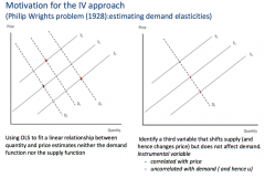
If the mean independence assumption does not hold, then E[uᵢ|Xᵢ] = 0 and therefore:

- the OLS estimator is unbiased and inconsistent

To mitigate this and obtain a consistent estimator, we can use an instrumental variables regression.

An Instrumental Variables regression takes a linear regression model:

Yᵢ = β₀+β₁Xᵢ + uᵢ, where E[uᵢ|Xᵢ] ≠ 0

- it then adds an additional variable Zᵢ (an instrument)

- This instrument isolates the part of Xᵢ that is uncorrelated with uᵢ (since this is what is needed to mitigate the failure of the mean independence assumption)

- This uncorrelated bit is the function of Zᵢ (without its error part) in the reduced form (since before the Xᵢ bit had itself some error in there, and now the errors together have been removed into a separate error in the reduced form)

- The instrument will then be correlated with Yᵢ but uncorrelated with Xᵢ

Motivation: The Phillip Wrights Problem

- Wanted to trace out the demand curve to work out the elasticity of demand

- If you looked at price changes and then looked at quantities, you wouldn't get a demand function

- This is because a demand shock can instead cause a price change (reverse causality)

- Also the change in price, may be due to a change in supply (supply not being held constant either, i.e. both supply and demand can change at the same time)

- So can use an instrument (something that shifts supply), that changes price but does not affect demand

- This will be correlated with price, but uncorrelated with demand

Front 62

What is the difference between en endogenous variable and an exogenous variable in linear regression?

Back 62

Endogenous Variables: variables that are correlated with the population error term uᵢ

Exogenous variables: variables that are uncorrelated with the population error term uᵢ

Front 63

What is an instrument?

To be valid, what does it need?

Back 63

An instrument Zᵢ is something which initiates a causal chain:

- Zᵢ affects Xᵢ (the treatment variable of interest, e.g. schooling)

- Xᵢ affects Yᵢ (the outcome variable of interest0, e.g. earnings)

To be a valid instrument, Zᵢ needs to:

- be as good as randomly assigned

- affect Xᵢ (relevance)

- only affect Yᵢ through Xᵢ - (the exclusion restriction)

If it is as good as randomly assigned and only affects Yᵢ through Xᵢ, then there is also independence/instrument exogeneity

Front 64

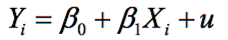
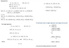
With IV with a single regressor and a single instrument, if Z is a valid instrument, what does β₁ in the population linear regression model measure?

What are the "first stage" and "reduced form" population linear regression models?

How do we obtain the "reduced from" population linear regression model?

Back 64

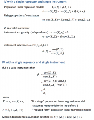
To obtain these models, start by just looking at Cov(Zᵢ, Yᵢ) and expanding it to get it in terms of β₁ and Cov (Zᵢ, Xᵢ)

(We use instrument relevance, so that we can divide both sides by cov(Zᵢ, Xᵢ).)

The numerator and denominator of β₁ are just like 2 population OLS estimators (from 2 particular linear regression models).

- each of these 'estimators' gives rise to the "first-stage" and "reduced form population linear regression models.

- the first stage linear regression model shows the relationship between the treatment variable and the instrument

- the reduced form linear regression model shows the relationship between the outcome variable and the instrument

- In both cases, the mean independence assumption of the error terms in these models holds

We obtain the "reduced form" population model by substituting in the "first-stage" population linear regression model into the original population linear regression model Yᵢ = β₀+ β₁Xᵢ + uᵢ

Front 65

What is the monotonicity assumption when dealing with an Instrumental Variable?

Back 65

Using the example of an instrument Z being a lottery (to be drafted) and treatment X being enlisted in the army. In the population:

- Always Takers - individuals who would enlist irrespective of the lottery outcome (proportion in population = pA)

- Never Takers - individuals who would evade draft irrespective of lottery outcome (proportion in population = pN)

- Defiers - individuals who would enlist if "unsuccessful in the lottery" but evade if they were "successful" (proportion in population = pD)

- Compliers - individuals who would enlist if they were successful in the latter, but no otherwise (proportion in population = pC)

Monotonicity Assumption:

- There are no defiers in the population!

- so pC = 0

Front 66

When dealing with an Instrumental Variable:

- In the reduced form linear regression model, what does λ₁ give us?

- In the first-stage linear regression model, what does π₁ give us?

- So what does β₁ give us in the original linear regression model?

Back 66

λ₁ is the LATE (i.e. the ATE for compliers) multiplied by the proportion of the population that are compliers:

- λ₁ = E[Yᵢ (1) - Yᵢ (0)|C].pC

µ₁ is the proportion of the population that are compliers:

- µ₁ = pc

So β₁ = λ₁/µ₁ = E[Yᵢ (1) - Yᵢ (0)|C] = LATE

- i.e. the ATE within the complier population

- it is a causal effect

Front 67

What is the two-stage least squares estimator (TSLS)? Are there any caveats to its use?

What are the 2 stages, intuitively?

What are the 2 stages, mechanically/formally?

Back 67

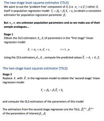
Using a two-stage least squares estimator (TSLS) is a way of obtaining a concisest estimator of the regression parameter β₁ in the context of a linear regression model?

- Caveat: it only works/is restricted to linear regression models, so it less general than the LATE that comes from using an IV

- They are the OLS estimators in the second stage linear regression model

Intuitively:

Stage 1: Decompose the regressor X into 2 components:

- A component that is uncorrelated with the error term (exogenous)

- A component that is correlated with the error term (endogenous)

Stage 2:

- Use the component that is uncorrelated with the error term (exogenous) to obtain an estimator of the regression parameter

Formally (shown in picture above):

Stage 1:

- Obtain the OLS estimators of parameters in the "first stage linear regression model

- Using these OLS estimators, compute the predicted value Xᵢˆ

Stage 2:

- Replace Xᵢ in the linear regression model with Xᵢˆ to obtain the "second-stage" linear regression model

- Compute the OLS estimators of the parameters of this model

- The estimators from this second-stage regression are the TSLS estimators

Front 68

What is the TSLS estimator formally in terms of X and Z?

By the LLN and CLT, what properties does it have?

Back 68

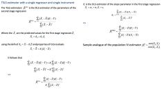
As normal, this βᵢᵀˢᴸˢ can be found in terms of its dependent/explanatory variables by doing (X-X¯) = some function of (Y-Y¯)

...but then rearranging in terms of Z...

... we end up with:

βᵢᵀˢᴸˢ = sample cov(Z, Y) / sample cov(Z, X)

- i.e. it is the sample analogue of the population IV estimator

Properties:

- by the LLN, the sample variance is a consistent estimator of the population variance

...so βᵢᵀˢᴸˢ →ᵖ β₁(where βᵢᵀˢᴸˢ is the sample mean of IID variables)

- and so by the CLT, it has a normal distirubiton in large samples

Front 69

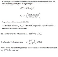
What is the sampling distribution of the TSLS estimator?

(I am not sure you really have to know this, but I've put it in for my notes/own reference...)

Given that the CLT theorem applies, what is its standard error, and t-statistic?

Back 69

Front 70

What is the man restriction in a General IV Regression model?

What does it mean for regression parameters to be exactly identified or over-identified?

Back 70

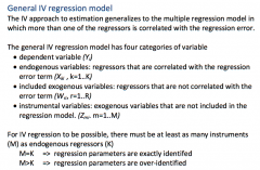
There must be at least as many instruments as endogenous regressors!

- Exactly identified: there are as many instrument as endogenous regressors

- Over-identified: there are more instruments then endogenous regressors

Front 71

Discuss Instrument Validity in the General IV Regression model

Back 71

Instrument Relevance:

- Intuitively: instruments must provide enough information about the exogenous variation in each of the endogenous regressors to sort out their separate effects on Y

- For each endogenous regressor X, at least one instrument Z must be useful for predicting X conditional on the exogenous regressors W

... i.e. in the first-stage regression, at least one of the instruments should be statistically significant

- The more of the information in X that is explained by the instruments, the more information is available to compute the IV estimators.

- So in many ways, having a more relevant instrument is like having a larger sample size

e.g. If the normal distribution is to provide a good approximation to the sample distribution of the TSLS estimator (like in the CLT when is is large), the instruments need to be highly relevant

- Also, when there are many endogenous regressors, we need to rule out perfect multicollinearity in the second stage regression

... i.e. no perfect linear relationship between the predicted values of the endogenous regressors and the exogenous regressors (including the constant term)

Instrument exogeneity:

- Each instrument is uncorrelated with the regression error, i.e.

Cov(Z₁ᵢ, uᵢ) = Cov(Z₂ᵢ, uᵢ) = ... = Cov(ZMᵢ, uᵢ) = 0

- If instruments are not exogenous, then the TSLS estimator is inconsistent

Front 72

What is a weak instrument?

What would this imply for the TSLS estimator?

How would you check for weak instruments?

Back 72

A weak instrument explains little of the variation in Xᵢ

If instruments are weak, then TSLS is no longer a reliable estimator.

- the normal distribution will provide a poor approximation to the sampling distribution of the TSLS estimator, even if the sample size is large, so there is no basis for statistical inference

- the TSLS estimator can be badly biased and 95% confidence intervals constructed in the usual way can contain the true parameter value far less than 95% of the time!

Front 73

How would you check for weak instruments?

Back 73

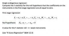
Just an F-test

- Where H₀ is that all coefficients on the instruments in the first-stage regression are zero

Front 74

How would you check for instrument exogeneity?

Back 74

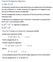
Instrument exogeneity:

- Each instrument is uncorrelated with the regression error,

... i.e.Cov(Z₁ᵢ, uᵢ) = Cov(Z₂ᵢ, uᵢ) = ... = Cov(ZMᵢ, uᵢ) = 0

- If instruments are not exogenous, then the TSLS estimator is inconsistent

- There is no direct test for instrument exogeneity

- But if the regression parameters are over-identified (i.e. there are more instruments than endogenous regressors) then theres an indirect test

Over-Identifying restrictions test (J Test)

- Suppose there is a single endogenous regressor X and two instruments Z₁ and Z₂

- You can compute two different TSLS estimators, one using Z₁ and one using Z₂

- if both instruments are exogenous, then the values of the two TSLS esimtators should be closed to each other

- but if the two TSLS estimators are very different, then there is a problem with the method

(Note: if regressors are exactly identified, then you can only get one TSLS estimator and the test cannot be used)

Or there is the Hausman method (See above)

- This compares the OLS estimator to the IV estimator

Front 75

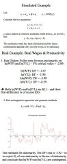
What is the benefit of doing both cross-section and time-series data?

Given a famous example.

Back 75

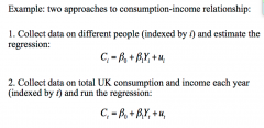
Note: The estimated β₁ is the MPC.

They may both be perfectly sense ways of looking at the relationship. Often by doing both, you learn something new from the different data.

Example: Kuznets Puzzle

- Cross-section shows MPC declining as income rises

- Time-series shows roughly stable MPC as income rises

Front 76

What is the main reason for using time-series data as opposed to cross-sectional data?

Why does the length of time chosen matter?

Back 76

They vary across time but not across individuals.

Cross-section data (indeed any data) requires variation in both the dependent and explanatory variables.

- both many variables are the same for each individual (e.g. GDP growth rate, world trade, etc.)

... this is true for all macro variables

- so to get variation, we exploit the fact that they change over time

Length of time for macro-series data:

- more time means more possible variation

- more variation, means we are better able to measure any effects

- e.g. it is possible to use just 3 data points and estimate an incorrect relationship from it

... this would be more unlikely if we examine more (/all) data

Front 77

What is important for time-series data to be "nice"?

Back 77

We should only consider consecutive, evenly-spaced observations

- e.g. monthly, 1960-1999, with no missing months

This is because missing and unevenly spaced months introduce technical complications.

Front 78

What is the first lag of a time series?

What is the first difference of a time series?

How would we find the percentage change from one period to the next?

Back 78

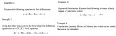
The first lag of a time series is its value in the previous period, i.e. Yt₋₁.

The first difference of a time series is the change in the level between the previous period and the current period, i.e. ΔYt = Yt - Yt₋₁

For the percentage change:

- divide the first difference by the first lag

- multiply by 100%

... i.e. 100 x (ΔYt / Yt₋₁)

- for small percentage changes, we can approximate this by 100ΔlnYt

Front 79

What is autocorrelation (or serial correlation)?

- what is it intuitively?

Notationally, what is:

- the first autocovariance of Yt?

- the first autocorrelation of Yt?

What about the jth sample autocorrelation?

- what makes it different to sample conventional correlations?

Back 79

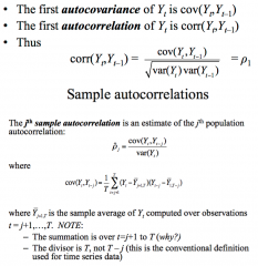
Autocorrelation:

- series with its own lagged values

- Intuitively: autocorrelation is present when a variable is consistently/consecutively above its mean, or consistently/consecutively below its mean

- The value of the time series today is therefore strongly correlated with its value last period (and sometimes periods before)

Note: These are population (not sample) correlations:

- they describe the joint distribution of (Yt, Yt-1)

- we could also generate the jth autocorrelation i.e. between Yt and Yt-j

Sample autocorrelation:

In the covariance term:

- We sum over t = j + 1, to t = T

... this is because we only start summing once we have enough data, i.e. for the first j pieces of, data Yj doesn't exist yet

- We divide by T, and not T-j

... this is because we do not correct for degrees of freedom in time series

Front 80

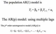
What is an autoregression?

What is the intuition for it?

What is the order of the autoregression?

Back 80

Autoregression:

- a regression model in which Yt is regressed against its own lagged values

- Intuition: Many macroeconomic variables have non-zero autocorrelations, so it makes sense to model economic time series against its past values

The order of the autoregression:

- the number of lags used as regressors

- i.e. in a pth order regression, Yt is regressed against Yt-1, Yt-2,..., Yt-p

β should be positive and significant if there is a strong autocorrelation.

Front 81

In the first-order autoregressive model: AR(1):

- what are the interpretation of β₀ and β₁?

How would we estimate the AR(1) model?

What about the coefficients in the AR(p) model?

Back 81

β₀ and β₁ do not have causal interpretations. It just tells us the relationship in the data.

- If β₁ = 0, then Yt-1 is not useful for forecasting Yt

- Testing β₁ = 0, vs. β₁ ≠ 0 provides a test of the hypothesis that Yt-1 is not useful for forecasting Yt

Estimating the AR(1) model:

- Performing an OLS regression of Yt against Yt-1

- (just as you would expect in a normal regression, button with a lagged variable instead of a new variable)

In the AR(p) model:

- Again, the coefficients do not have a causal interpretation

- To test the hypothesis that Yt-2,..., Yt-p have of not further help forecast Yt beyond Yt-1, use an F-test

Front 82

What is an ADL model?

How does whether we are forecasting or just describing Y change whether we include the present value of X?

Back 82

An ADL model is an autoregressive distributive lag model.

- as well as forecasting models that use past values of the forecasted variable, it also includes lags of other variables (that might also be useful predictors of Y)

An autoregressive model with p lags of Y and r lags of X:

- ADL (p, r)

If we are forecasting Yt:

- we cannot include Xt, since we don't know it yet, i.e. it is observed at the same time as Yt

But if we are just being descriptive:

- then we can include Xt

Front 83

How should we decide whether to include lagged X's to predict Y?

- i.e. to convert an AR model into an ADL model?

What do we have to be wary of about the name of this test?

Back 83

Use a Granger Causality Test

- This test whether the set of lagged X's should be included in addition to the lagged Y's

- This is simply an F-test of the hypothesis that all the estimated coefficients on the lagged X's are equal to zero,

... i.e. H₀: δ₁ = δ₂ = ... = δᵣ = 0

But this test is not really a "causality" test:

- there is no randomised control experiment

- we are just testing whether X"s have marginal predictive power, i.e. whether previous va;lies of X do or do not affect current values of Y

Front 84

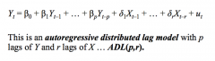
What is the difference between "in-sample" values and "out-of-sample" values in time-series data regression?

What are the AR(1) forecast model, in both population and sample terms?

What is a forecast error and how is it different to a residual?

Back 84

In-sample values - are just predicted values (i.e. we have the data and already know the outcome, but want to see what our model gives us).

Out-of-sample-values - are forecasts into the future - we don't know what the true value should yet be.

Note: YT+1|T means a forecast of YT+1 given everything we know up to time T.

- The population version uses the population (true unknown) coefficients

- The sample version uses estimated coefficients... i.e. it is what we do in the real world

The one-period ahead forecast error is the difference between actual income and what we predicted it would be:

- The forecast error is "out-of-sample", i.e. the value of YT+1 is not used in the estimation of the regression coefficients

- but a residual is "in-sample"

Front 85

Why do we need a measure of forecast uncertainty?

What is the forecast error in the model above?

Can this be split into two types/sources of errors?

Back 85

We need a measure of forecast uncertainty to:

- construct forecast intervals

- let users of your forecast know what degree of accuracy to expect

Two sources of error:

- First term: uT+1: True uncertainty in the world. This is the main problem. This is the simple fact that there is always error, since stuff happens that you could never have forecasted (by definition), e.g. shocks to oil price

- Second term in square brackets: True uncertainty in the model: the error caused by the fact that our beta estimates are not the true population parameters.

...This is less of a problem, since if n is large, then are sample parameters will be close to their true population values

Front 86

What is the Mean Squared Forecast Error?

What is the Root Mean Squared Forecast Error?

Back 86

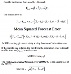
It does what it says on the tin:

- take the forecast error (which is itself broken down into two parts: the true uncertainty in the world, and the uncertainty in the model)

- square it

- then take the mean

So MSFE = var(uT+1) + uncertainty arising because of estimation error

- but if the sample size is large, then this second uncertainty effect from the estimation error is (much) smaller than var(uT+1),

so MSFE ⋍ var(uT+1)

The RMSFE, is just the square root of the MSFE

- it is a measure of the spread of the forecast error distribution

- it is like the standard deviation of ut, except that it explicitly focuses on the forecast error using estimated coefficients, not using the population regression line

- it is a measure of the magnitude of a typical forecasting "mistake"

Front 87

What is POOS forecasting and why is it used?

How can you use this to generate the MSFE?

Back 87

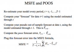
POOS Forecasting is Pseudo Out-Of-Sample Forecasting:

- It is a method for simulating the real-time performance of a forecasting model

- You pick a date near the end of the sample and estimate the mode using data up to that data.

- You then use that estimated model to make a forecast, for which you can immediately calculate the forecast error

- You can then repeat this with multiple dates near the end and generate a series pf pseudo forecasts and thus pseudo forecast errors

- This means that you can see what sort of forecast errors the model will produce without having to use it for real

- You can then plug this into the MSFE formula, to work out what you expect the MSFE to be, before that period actually occurs

Front 88

What is a forecast interval - how can it be constructed?

Why is it not a confidence interval?

What is a common forecast interval to use?

Back 88

A forecast interval is an estimated range of values a random variable could take at some point in the future.

If uT+1 is normally distributed, then a 95% forecast interval can be constructed as:

YˆT|T+1 ± 1.96 x RMSFE

(but it is only valid if uT+1 is normal).

It is not a confidence interval:

- Since YT+1 is random - the interval helps us to estimate an unknown future value of a random variable

- By contrast, a confidence interval usually applies to fixed (but unknown) estimates of parameter values

It is common to use a "67%" forecast interval,

... i.e. ± 1 x RMSFE = ± RMSFE

- this covers a smaller percentage of the bell-shaped curve

- this a result of how difficult forecasting is - it is almost impossible to be correct 95% of the time

Front 89

How if forecast uncertainty used in practice by the BoE?

What determines the shape of fan charts?

Back 89

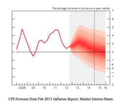
The BoE produces quarterly forecast for Inflation (and GDP growth) in the Inflation Report. This consists of:

- the central projection: the modal forecast for inaction, i.e. the most likely path the BoE thinks inflation will take

- the fan charts: the forecast uncertainty/interval

Problems:

- very wide forecast intervals, i.e. even one-month ahead forecast's 90% forecast interval can span 5 percentage points of inflation

Fan charts are the probability distributions of future inflation. Their share reflects:

- the central projection (the mode), which determines the profile of the central darkest band

- The degree of uncertainty, which determines the width of the fan charts (i.e. bigger RMSFE)

- The position of the mean relative to the mode (the choice of the CB - using private information and how models have actually done in the past), which determines whether fan charts are symmetrical or skewed

Forecasting is generally more accurate when the economy is stable.

Front 90

Manipulate these time-series equations:

Back 90

Front 91

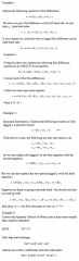
Does instability in model parameters matter?

How does statistical significant different from quantitative/economic significance?

What is an impulse response function?

Back 91

If the model is not stable, you can't really forecast it? This is an empirical matter...

Statistically significant (e.g. significant t-rest result) result can occur even if it quantitatively/economically insignificant.

This means the data/result can explain something but has a tiny coefficient, so it can be ignored.

Implies response function:

- Too see this, think of sending a shock (i.e. a change in et in the model above)

- then plot the subsequent responses on inflation)

- this may be different for two different time periods, implying that a parameter has changed over time.

- but we can see that although it has changed, this change has not made a huge difference to the model

- but this is not always the case - it may depend on the variable

Front 92

In reality, how do we predict inflation?

Can we outperform the AR(1) model?

Back 92

We can use different methods, e.g.

- Using unemployment (e.g. the Phillips Curve

- Using other real activity measures

A simple solution:

- combine all the activity indices into one

- weight each by their usefulness in forecasting inflation

We could also use other variables other than those which directly measure real economic activity, e.g.

- Interest Rates (yield curve slope)

- Monetary Aggregates

- Stock Market Returns

- House Prices

- Exchange rates

... but so far, these have not reliable forecast inflation

It is difficult to beat simple univariate AR model of inflation as a forecasting tool?

- To the extent that we can outperform AR models, we need to combine indices (shown above) or alternatively combine forecasts from models with different indices

Front 93

How can we compare/evaluate there performance of two forecasting models?

Back 93

We can compare the RMSFE (Root mean Squared Forecasting Errors).

Or we can calculate the RMSFE ratio.

RMSFE(A)/RMSFE(B) < 1, implies that model A is better at forecasting.

Front 94

What is a stationary time series?

What is a non-stationary time series?

What does this mean intuitively?

Back 94

A time series Yt is stationary if:

- its probability distribution does not change over time

- i.e. the joint distribution of (Ys+1, Ys+2, ..., Ys+T) does not depend on s regardless of the value of T

- i.e. no matter how many periods in the time series, the probability distribution over any period is the same

- Intuitively: historical relationships based on past data are useful in forecasting the future

A time series Yt is non-stationary if:

- its probability distribution does vary over tome

- Intuitively: the future differs fundamentally from the past, so historical relationships may not be a good guide to the future

Front 95

What are two sources of non-stationarity?

Back 95

Two Sources of Non-stationarity:

- Trends

- Structural Breaks

Front 96

Trends

Is a trend a source of stationarity or non-stationarity?

What is a trend?

- what are the different types of trends?

- In general, are economic time-series driven by one of these trends?

- what does it mean for a the first-difference to be trend-free.

What are the important points/key features of a random walk?

How would we augment the random walk model with drift?

Back 96

Trends are a source of non-stationarity.

Trends:

- A trend is simply a persistent long-term movement of a variable over time

- Most macro time-series variables have a trend, with annual observations then fluctuating around this trend

Trend Type 1: Deterministic Trend

- A trend that is a non-random function of time

e.g.Yt = α + βt for t = 1, 2, 3...

- Then Yt grows at the rate β, since one period later, Yt+1 = α + β(t+1) = a + βt + β = Yt + β

- Subtracting Yt from both sides gives us the first-difference...

Yt+1 - Yt = ΔYt+1 = β

... the first different of Y is constant - so is trend free

- In general, economic time-series are probably not driven by a deterministic trend

... the internet predictability of a deterministic trend is hard to reconcile with events such as the productivity slowdown or the Great Moderation

... trends do exist, but they surely have a substantial unpredictable (random) component

Trend type 2: Stochastic Trend

- The simplest model of a variable with a stochastic trend is the random walk

... The random walk (with or without drift) is a good description of stochastic trends in many economic time series

- A time series Yt follows a random walk, if:

Yt = Yt-1 + ut (where ut is a random shock, which we can assume is distributed ut ~ IN[0, σ²u], i.e. an independently distributed normal random variable with a mean (expected value) of zero, so:

... E[ut] = 0 and Var[ut] = E[u²t] = σ²u

- The basic idea: the value of the series tomorrow is its value today plus an unpredictable change.

... the path followed by Yt therefore consist of random steps ut

... so that path is a random walk

- The first difference of this variable is ΔYt = ut, so the first difference is now also random

The Random Walk's key features:

- YT+h|T = YT

... i.e your best prediction of the value of Y in the future is the value of Y today

... e.g. to a first approximation, log stock prices follow a random walk (I.e. stock returns are unpredictable.. but our best guess for the price tomorrow is just the price today)

- Suppose Y0 = 0. Then Var(Yt) = tσ²u

... i.e. the variance depends on t, so variance increases linearly with t

... so Yt cannot be stationary, and its distribution depend on the value of t

The Random walk with drift:

- Yt = β0 + yt-1 + ut (where ut is serially uncorrelated)

... β₀ is the "drift". If β₀ ≠ 0, then Yt follows a random walk around a linear trend

- e.g. in the "h-step ahead" forecast, our best guess of Y in the future is its value today plus the effect of the trend over time

... YT+h|T = β₀h + YT

Front 97

How does the random walk (with drift) relate to an AR(1) model?

Back 97

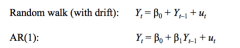
The random walk is just an AR(1) model with β₁ = 1

- This special case where β₁ = 1 is called a unit root

- We also say that the series is integrated of order 1, or ... I(1)

- so in the AR(1) model, when β₁ = 1, to becomes

ΔYt = β₀ + ut

Front 98

What are some problems caused by trends?

How can we mitigate these problems caused by trends?

Back 98

1. AR Coefficients are strongly biased toward zero.

... this leads to poor forecasts

... if Yt really does follow arandom walk, then forecasts based on the AR (1) model with a biased β₁ can perform substantiallyworse than those based on the random walk model which imposes the true value of β₁ = 1

2. Some t-statistics don't have a standard normal distribution, even in large samples

... so conventional confidence intervals are not valid and hypothesis testscannot be conducted as usual.

... An important example of this problem arises inregressions that attempt to forecast stock returns using regressors that couldhave stochastic trends

3. If Y and X both have random walk trends then they can look related even if they are not, i.e. you can get "spurious regressions"

... e.g. US and Japanese GDP may rise at the same time

... these then conspire to produce a regression that appears to be significant

... but there is no compelling economic/political reason to think that the two series are related, i.e. they are spurious

Mitigating these problems:

- eliminate the trend in Yt by eliminating it and working with the first-difference

Front 99

How can we test for stochastic trends in the AR(1) model?

How can we test for stochastic trends in the AR(p) model?

What is a problem with these tests in practice?

Back 99

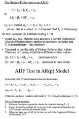
We can run the regression of the random-walk specification and test the significance of the coefficient.

This is the Dicker-Fuller Test in AR(1)

- take a population linear regression model and test for non-stationarity, (i.e. β₁ = 1)

- subtract Yt-1 from both sides to get the equation in terms of the first lag and δ = (β₁ - 1)

- H₀: β₁ = 1 (there is a unit root, i.e. the series is non-stationary), H₁: β₁ < 1 (the time series is stationary) ... rearranging in terms of δ enables us to use the null as equation something to zero

... note that this test only has to be one-sided

The DF Test:

- Under H₀, this t-statistic does not have a normal distribution (since that would only apply to stationary variables but Yt is non-stationary here under H₀)

- Use the table of DF critical values, for which there are two cases

... case 1: intercept only

... case 2: intercept and time trend

This is the Augmented Dicker-Fuller Test for AR(p):

- Now we rewrite the model as above

- The same principle applies, i.e. if there is a unit root, than δ = 0, and there is a random walk trend

- Estimate the regression and obtain the t-statistic under H₀: δ = -

- Reject the null of a unit root if the t-stat is less than (i.e. more negative than) the ADF critical value

Dickey-fuller tests in practice

- So if Yt has a unit root (we could not reject H₀), then it makes sense to avoid the problems this poses by modelling Yt in first differences, i.e. ΔYt

- but in practice, the Dickey-fuller test have low power

... i.e. if the true coefficient is 0.98, then the series stationary,

... but you may not reject non-stationarity in the data (i.e. you may conclude non-stationarity)

... this is because the data sample is finite, and so may not be able to tell the difference between a unit-root, and a stationary-process with a near-unit root

Front 100

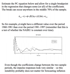
Structural Breaks

What is a structural break?

How would you test for a break (change) in coefficients?

Back 100

A structural break is:

- when the coefficients of the model might not be constant over the full sample

... it is clearly a problem fore forecasting if the model describing the historical data differs from the current model, since you want the current model from your forecasts

... this would be an issue of external validity

- it is another source of non-stationarity

- this occurs often in economic, e.g. when there is a change in economic policy, or when there is new invention

Testing for a break change depends on whether the break date is known or not.

When the break date is known:

- Say it occurs at date 𝛕, e.g. you know when the exchange rate regime changes

- then the stability of the coefficients can be tested by estimating a fully interacted regression model.

In the ADL(1, 1) model:

- if the new parameters ɣ₀ = ɣ₁ = ɣ₂ = 0, then the coefficients are constant over the full same

- but if at least one of the gamma terms are nonzero, then the regression functions changes at date 𝛕

To test the hypothesis that these gamma terms are all zero, obtain the Chow test statistic for a break at data 𝛕 - this is the (heteroskedacity-robust) F-stasistic. This is tested against the alternative hypothesis that at least one of the gamma terms are nonzero.

Also:

- also, you can apply this method to a subset of the coefficients if needed, e.g. only the coefficient on Xt-1

- unfortunately though.... you often do not have a candidate break date... (i.e. you do to always know 𝛕)

Front 101

What is co-integration?

How would you eliminate what the variables in question have in common?

How would you test for cointegration?

When is the OLS estimator of the coefficient in the cointegrating regression consistent?

Back 101

If Xt and Yt are cointegrated, they have the same (or common) stochastic trend.

- Computing the difference Yt - θXt eliminates this common stochastic trend.

Suppose Xt and Yt are integrated of order one, I(1). If for some coefficient, θ, Yt - θXt is integrated of order zero, I(0), then Xt and Yt are said to be cointegrated.

The coefficient θ is called the cointegrating coefficient.

Testing for Cointegration

1. Test the order of integration of both variables, X and Y

2. If they are the same, then estimate the cointegration coefficient

3. Test the residuals (Yt - θXt) for stationarity using the Dickey-Fuller test.

Note that if the two time-series ARE cointegrated, then the OLS estimator of the coefficient in the cointegrating regression is consistent.

- However, in general the OLS estimator has a non-normal distribution and inferences based on t-stats can be misleading.

Front 102

What is the error correction model?

What is its economic intuition?

Back 102

If Xt and Yt are cointegrated, then a way of eliminating the common trend (to mitigate the problems that trends cause), is to compute Yt - θXt, where θ is the cointegrating coefficient that eliminates the common trend.

The Error correction model is just the ADL model with the addition of the Error Correction term.

- the error correction term can be used in regression analysis because it is stationary!

- since Yt and Xt are I(1), their first difference is also I(0).

- So all the variables in this model are I(0)

Economic intuition:

- If a shock temporarily moves Y away from its long-run relationship with X...

- then the ECM term shows that over time this discrepancy will be reversed (since α < 0 in this model)...

- so Y will move back toward the equilibrium relationship with X

- so this amended ADL model has a long-run solution (where there is no change in Y or X, so ΔY and ΔX are zero) - this is just the long-run cointegrating relationship

Front 103

What is the intuition behind excess smoothness (if permanent income is less smooth than current income)?

Back 103

- If Yt is non-stationary, then an innovation at time t does not cause a temporary deviation of income from trend, but has a permanent effect on the level of Yt

- So any innovation to income is an innovation to permanent income

- But the PIH states that consumption is determined only by this permanent income

- So if permanent income is less smooth than current income

- then consumption should be (less smooth) more volatile than current income too

- but in the data, consumption is only 0.64 times as volatile as income

- So consumption is in fact excessively smooth

Front 104

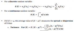
What is the formula for:

- the mean of a discrete random variable

- the mean of a continuous random variable

What about the variance?

Back 104

Front 105

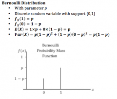
Bernoulli Distribution

What its mean?

What is its variance?

Back 105

Front 106

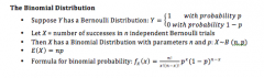
Binomial Distribution

- What is the formula for binomial probability?

- What is the mean?

- What is the variance

Back 106

Front 107

Normal Distribution

- What is the formula for P(X = x), i.e. f(x)

Back 107

Front 108

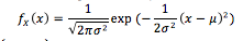
What is the formula for skewness and Kurtosis?

What is the skewness and Kurtosis of the standard-normal distribution?

Back 108

Front 109

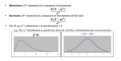
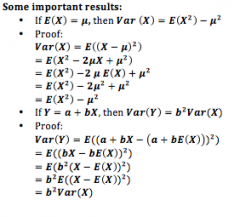
Prove that E(a + bX) = a + bE(X) for a continuous random variable?

Back 109

Front 110

If E(X) = µ, show that Var(X) = E(X²) - µ²

If Y = a + bX, show that Var(Y) = b² Var(X)

Back 110

Front 111

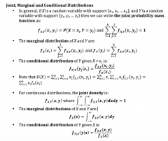
For Discrete Random Variables:

- What does the joint probability mass function of x and y look like?

- What does the marginal distribution of x and y look like?

- What does the conditional distribution of x and y look like?

For Continuous Random Variables:

- What does the joint probability density function of x and y look like?

- What does the marginal distribution of x and y look like?

- What does the conditional distribution of x and y look like?

Back 111

Front 112

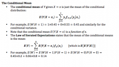
What does the conditional mean of Y given X look like mathematically?

What about the Law of Iterated Expectations?

Back 112

Front 113

What is the condition for independence of events?

What does this imply for covariance?

- Is this relationship one way?

What is the formula for correlation?

Back 113

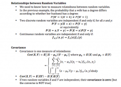
The Covariance relationship is one way:

- If two independents are independent, then their covariance is 0

- but the converse is not necessarily true

Correlation:

- Corr(X, Y) = Cov(X, Y)/√(Var(X)Var(Y))

- It is possible for correlation to be zero even if X and Y are perfectly related, if the relationship is collinear

- This is because correlation measures a linear relationship

Front 114

What is the Bivariate normal distribution?

Back 114

Front 115

What is a Random variable?

What is a simple random sample?

- what does this imply for IID-"ness"?

Back 115

Front 116

What is the probability distribution of the sample mean, if the sample is IID?

What is this distribution called?

Back 116

This is called the sampling distribution of Y¯.

Front 117

What is an estimator?

What is an estimate?

What are the desirable characteristics of an estimator?

Back 117

- An estimator is any function of a sample of data drawn randomly from apopulation and is a random variable e.g. taking the first value drawn - An estimate is the numerical value the estimator takes in a specific sampleand is a non-random variable

- Unbiasedness - the mean of the sampling distribution equals the population mean

- Consistency - the sample mean converges in probability (as n increases) to the population mean

... in other words, when the sample size is large, uncertainty regarding the value of the population mean arising from random sample variation is small

- Efficiency - when comparing two unbiased estimators, the one with the lowest variance if more efficient than the other

Front 118

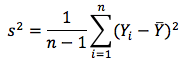
What is the formula for sample variance?

Back 118

Front 119

Intuitively, what is the standard error of the estimate?

What is the standard error of a Bernoulli estimate?

Back 119

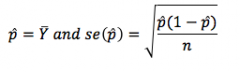
It is a measure of how far away the estimate might be from the true value.

Front 120

What is real equivalised household income?

What are the problems with it?

Back 120

Xᵢ = Yᵢ (Pᵢ /Cᵢ)

- Y is nominalhousehold income, measured in the Family Resources Survey

- P ismeasured/approximated by the RPI

- C is measured/approximated by a modified OECD equivalence scale (there is a bit of variationfor different income measures)

Problems:

- Taste variation cannot always be explained by variation in characteristics

- This does not account for externalities, non-market goods, home-production, etc.

- There is also no discussion of savings or sit

Front 121

What is a Kolmogorov Smirnov Test?

Back 121

- This compares a hypothesised population CDF and another empirical sample CDF, to see if they are the same

- It takes the largest difference between the CDFs at any x-value as the test-statistic

- It has its own set of critical values

- Reject if the gap between the CDFs is bigger than the critical value

- At 5% significance level, then if the null is true, only in 5% of random samples of this size would we expect to see a maximum absolute deviation between the empirical sample CDF and the theoretical population CDF of the size of the critical value for 5%

Front 122

Why does the lognormal test generally fail to accurately represent income and wealth distributions?

Back 122

Income and wealth distributions generally have "fat tails"

- i.e. high incomes occur more often than you would expect from a normal model

Front 123

What are two simplifications used with social welfare functions?

What are three different social welfare functions?W

Back 123

Simplifications:

- Fixed population size

- Abstracting from efficiency (??? - bloody second year notes)

Possible SWFs:

- Benthamite/utilitarian (ignoring inequality, caring only about utility, which is assumed to be motivated by income)

- Rawlsian: only cares about poorest person in society

- Generalise Utilitarian

Front 124

What are the properties of a desired social welfare function?

Back 124

1. Pareto Condition (Monotonicity)

- Welfare must be increasing in all welfare arguments

- (e.g. making one person better off, assuming no one is made worse off, is preferred)

2. Anonymity (symmetry in diagonal line)

- Swap the wealth of a rich and poor person and SWF remains unchanged

3. Principle of Transfers/Dalton's Principles/convexity to origin

- Transfer of income from a richer person to a poorer person will increase equity

... provided the ranking of the two is not preferred by the transfers

- basically the "averages are preferred to extremes" argument

4. Homogeneity of degree 1:

- Multiplying everyones income by factor k

- Multiplies overall welfare by k

Front 125

What is a possible (very generalised) way of measuring inequality in an income distribution?

How can we then write social welfare notationally?

Back 125

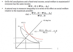
Measuring it relative to perfect equality.

Then: W = x¯( 1- i(x) )

But the choice of inequality measure implies a certain value judgement about the kind of inequality which matters to you in your swf.

Front 126

Write the functions of the following inequality measures:

- Range

- 90/10 ratio

- Variance

- Mean absolute deviation

- Coefficient of Variation (defined as a ratio of what)

- Entropy

- Gini Coefficient

Back 126

Front 127

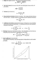
What is the Atkinson Index? What is it useful for?

What does epsilon represent?

Back 127

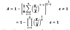
This is a measure of inequalitydeveloped by British economist Anthony Barnes Atkinson. This measure is usefulin determining which end of the distribution contributed most to the observedinequality.

Epsilon measures the inequality aversion parameter. (must be ≥ 0)

- For a higher epsilon, the index is more sensitive to changes in the lower end of the income distribution

- For a lower epsilon, the index is more sensitive to changes in the upper end of the income distribution

Front 128

How are measures of poverty different to SWFs?

What affect does the poverty line have for poverty measures?

How is the poverty line chosen?

Back 128

Poverty measures account only for changes in poverty, i.e. those below a 'poverty line'.

The poverty line has the following effects:

- assigns zero significance to an increase in welfare of the non-poor – itdoes not affect poverty

- Gives zero weight toinequality-reducing transfers within sectors e.g. within poor, or within non-poor population

Poverty line choice is tricky:

- In UK: 60% of median income

- In US: based on dollar amount needed to buy 3 low cost food plans

Front 129

Name 3 Poverty Measures, and what they measure.

Back 129

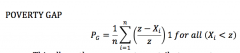
1. Headcount

- Measures proportion of population below poverty line

- It is the value of theempirical CDF at z (i.e. the poverty line income)

- This could be a SWF if peoplebelow z are weighted -1 and peopleabove z are weighted 0. ... It is monotonic increasing in x but it is not concave andviolates the principle of transfers.

2. Poverty Gap:

- This allows the very poor tocontribute more to measured poverty that the not-so-poor.

- It is interpretable as a percapita measure of the total shortfall of the households below the poverty line.

- The implied SWF is increasingin x and (just) concave –satisfies monotonicity and quasi-concavity

3. Sen's Poverty Index

- This index is meant to addressthe shortcomings of the poverty ga, and accounts for mean income amongst the poor

- Gp is the Gini coefficient and x¯p is the mean income amongstthe poor.

- When there isn’t any inequalityamongst the poor, this reduces to the poverty gap measure. - - However, given it isbased on the Gini, it shares the Gini’s problems.

Front 130

What is Manski's Law of Decreasing Credibility?

Back 130

the credibility of inference decreases with thestrength of the assumptions maintained”.

Front 131

What assumptions do we need to make to rank income distributions more easily?

Back 131

1. Monotonicity

2. Concavity

If both CDFs are monotonic, and one is more concave then the other, then we can state First-Order Stochastic Dominance.

CHECK THIS IN NOTES - aren't ALL CDFs monotonic?

Front 132

What question is implied by: "is there Selection Bias"?

Can we know which direction it is?

Back 132

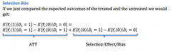
The selection bias asks thequestion: would we expect to see a difference in outcomes between the treatmentand non-treatment groups even if no treatment was applied?

We cannot know for sure a priori whether it is positive or negative.

In the exam argue for both, but perhaps say why one is more appropriate.

Front 133

What does a Randomised Control Trial imply for:

- potential outcomes?

- the ATT?

Back 133

Front 134

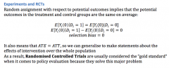
When does a study have internal validity?

- what are the threats to it?

When does a study have external validity?

- what are the threats to it?

Back 134

Internal Validity:

- A study is said to haveinternal validity if the statistical inferences about causal effects are validfor the population being studied

- Properly executed RCTs havehigh internal validity

- Internal validity has twocomponents:

.... The estimator of the causaleffect should be unbiased and consistent

... Hypothesis tests should havethe desired significance level

Threats to internal validity:

- Contamination: people in the control groupaccess the treatment anyway

- Non-compliance group: people in the treatment group refuse to take the treatment

- Hawthorne effect: participants alter their behaviour as a resultof being part of an experiment

- Placebo effect: participants alter their behaviour as a result of perceived changes, which affects final outcomes

Or in multiple regression analysis, interval validity can be threatened by:

- Omitted Variable bias: a variable that determines Yand is correlated with one or more regressors is not included

- Measurement error bias: when an independent variable is measuredimprecisely

- Sample selection bias: when a selection process influences availabilityof data and the process is related to the dependent variable

External Validity:

- A study is said to haveexternal validity if its inferences and conclusions can be generalised from thepopulation and setting studied to other populations and settings

- This generally requires an invariance assumption, i.e. thedistribution of outcomes would be the same under both the specific experimentaltreatment group and different populations

Threats to External Validity:

- Differences in populations: this can come through thesmall/local nature of an RCT that may only focus on a particular geographic ordemographic group – also animal testing leading to conclusion about treatmenteffect on humans?

- Differences in settings: even if populations are the same, institutionalenvironments may differ e.g. studying effect of advertising on binge drinkingmay not be useful to generalise due to different legal penalties or culturesetc

- Compliance problems: most RCTs employ volunteers whowill be more committed to undertaking treatment but other populations may notcomply with

- Short durations of studies: often we want to know LT outcomes of treatmentbut RCTs only reveal immediate outcomes

Front 135

In terms of bounds, what is the greatest value an ATE could take?

Back 135

Front 136

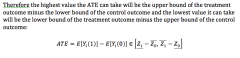
When is the Conditional Independence Assumption incredible?

What is a realistic problem with using it?

Back 136

If there is still randomisation even after conditioning on covariates: i.e. if there are still relevant some covariates which are not included.

To be plausible, you may need to condition on many covariates (i.e. zoom into a very small cell in the population). In this cell, there may not be many people in it to treat and control.

Front 137

What is an Instrumental Variable?

What qualities does it need to be valid?

What is the LATE?

- How do we work out the complier population to find the LATE?

Back 137

An instrument Z is a variable which initiatesa causal chain:

- Z affects D (the treatment variable ofinterest)

- D affects Y (the outcome variable ofinterest)

In order to be valid, it must satisfy the following properties:

- relevance - instrument must affect the decision variable D

- exogeneity - instrument must only affect the outcome variable Y through D

- it must be randomly assigned (i.e. orthogonal to treatments and potential outcomes)

- Monotonicity: there are no "defiers", i.e. there are no individuals for who take treatment when Z = 0, or refuse treatment when Z = 1

Then the instrument will be able to isolate the Local Average Treatment Effect (LATE) - LATE is shown above

- this is the ATE for the subgroup of compliers

- but if compliers are themselves a random selection of the population, then LATE = ATE

The problem is identifying thecompliers within the observable groups since those who satisfy the instrumentand treatment variable could also be Always Takers and those who satisfyneither the instrument variable nor the treatment variable could also be NeverTakers

- However since is randomly assigned, theproportions of each type of individual are the same in the and groupsTherefore, the proportion of Always Takers andNever Takers are

- So the proportion of always-takers are: P(D = 1|Z = 0)

- And the proportion of never takers are: P(D = 0 | Z = 1)

- The proportion of compliers is then just 1 - (these two proportions)