![]()
![]()
![]()
Use LEFT and RIGHT arrow keys to navigate between flashcards;
Use UP and DOWN arrow keys to flip the card;
H to show hint;
A reads text to speech;
56 Cards in this Set
- Front
- Back
- 3rd side (hint)
|
Consumer behaviour |
Description of how consumers allocate income among different goods and services to maximise their well-being. |
1 Consumer Behaviour |
|
|
Three distinct steps of consumer behaviour: |
1. Consumer preferences 2. Budget constraints 3. Consumer choices |
1 Consumer Behaviour |
|
|
Consumer preferences |
Describes the reason people might prefer one good to another. |
1 Consumer Behaviour |
|
|
Budget constraints |
Limited incomes restrict the quantities of goods people can buy. |
1 Consumer Behaviour |
|
|
Consumer choices |
Consumer preferences and budget constraints together (consumers choose to buy combinations of goods that maximize their satisfaction). |
1 Consumer Behaviour |
|
|
Market baskets |
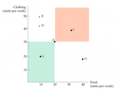
A list of specific quantities of one or more goods. (quantities of food vs clothes that consumer buys each month) Food Clothes A 10 10 B 5 15 C 13 7 |
1 Consumer Behaviour |
|
|
Preferences. Completeness |
Consumers can compare and rank all possible baskets. Consumer will prefer A to B, B to A or will be indifferent. |
1 Consumer Behaviour |
|
|
Preferences. Transivity |
Transivity is normally regarded as necessary for consumer consistency. If consumer prefers A to B and B to C, then consumer also prefers A to C. (Porsche is preferred to a Cadillac and aCadillac to a Chevrolet, then a Porsche is also preferred to a Chevrolet.) |
1 Consumer Behaviour |
|
|
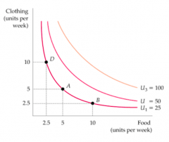
Indifference curve |
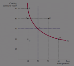
Curve representing all combinations of market baskets that provide a consumer with the same level of satisfaction.
|
1 Consumer Behaviour |
|
|
Indifference maps |
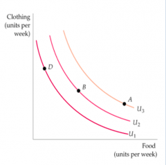
A set of indifference curves that describes a person's preferences. !! Indifference curves cannot intersect !! |
1 Consumer Behaviour |
|
|
Marginal rate of substitution |
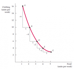
Maximum amount of a good that consumer is willing to give up in order to obtain one additional unit of another good. MRS = -ΔC/ΔF (change in clothes/change in food) MRS = -(-6)/1=6 |
1 Consumer Behaviour |
|
|
Shapes of indifference curves |
The shape of indifference curve describes the willingness of a consumer to substitute one good for another: 1. Perfect substitutes 2. Perfect complements |
1 Consumer Behaviour |
|
|
Perfect substitutes |
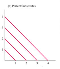
Goods are substitutes when the marginal rate of one for the another is constant. (1 glass of apple juice for 1 glass of orange juice) |
1 Consumer Behaviour |
|
|
Perfect complements |
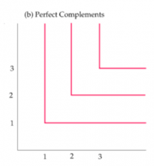
Goods are complements when one good increase satisfaction only if obtain the other good. (1 right shoe and 1 left shoe) |
1 Consumer Behaviour |
|
|
Utility |
Numerical score representing the satisfaction that consumer gets from a given market basket. |
1 Consumer Behaviour |
|
|
Utility function |
A set of indifference curves with a numerical indicator. u(F,C) = FC |
1 Consumer Behaviour |
|
|
The budget line |
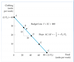
A budget line describes the combinations of goods that can be purchased given the consumer's income and the prices of the goods. PFF + PCC = I |
1 Consumer Behaviour |
|
|
Maximising consumer satisfaction |
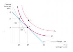
1. The basket must lie on the highest indifference curve that touches the budget line. 2. Satisfaction is maximised when MRS = PF/PC (marginal benefit = marginal cost) |
1 Consumer Behaviour |
|
|
Individual demand |
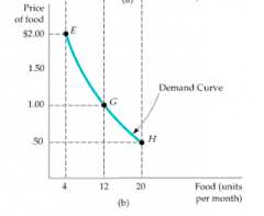
Curve relating the quantity ofa good that a single consumerwill buy to its price. |
2 Demand |
|
|
Engel curve |
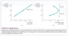
Curve relating to the quantity consumed to individual's income. |
2 Demand |
|
|
A fall in the price of a product has to effects: |
1. Substitution effect 2. Income effect |
2 Demand |
|
|
Substitution effect |

Change in consumption of a good associated with a change of its price. (utility held constant) |
2 Demand |
|
|
Income effect |

Change in consumption of a good resulting from an increaase in purchasing power (products are cheaper, so you can buy additional units of a good) (prices held constant) |
2 Demand |
|
|
Inferior good |
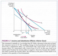
Substitution effect is bigger than income effect. (A good is inferior when income effect is negative.) (daugiau atpigusio maisto ir biski dar drabuziu) |
2 Demand |
|
|
Giffen good |
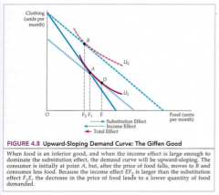
When good is an inferior good and the income effect is bigger than substitution effect. (nepirksiu atpigusio maisto, nusipirksiu daugiau drabuziu) |
2 Demand |
|
|
Normal good |
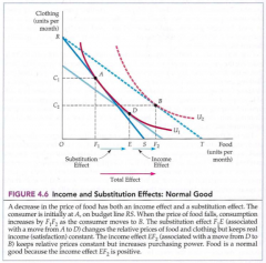
Income effect is the same as substitution effect (maistas atpigo tai pirksiu daugiau maisto ir tiek pat drabuziu) |
2 Demand |
|
|
Market demand |
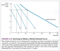
Shows how much all consumers are willing to purchase as its price changes. |
2 Demand |
|
|
Price elasticity of demand |
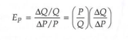
Measures the percentage change in the quantity demanded resulting from a 1 percent of increase in price. (kaip keicias paklausa nuo 1% didesnes kainos) |
2 Demand |
|
|
Probability |
Likelihood that given outcome will occur. |
3 Uncertainty/Risk |
|
|
Expected value |

Probability-weighted average of the pay-offs associated with all possible outcomes. |
3 Uncertainty/Risk |
|
|
Variability |
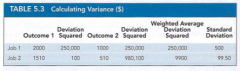
Extent (size) to which possible outcomes of an uncertain event differ. 1. Find Deviation (0.5 x 1000 + 0,5 x 2000 = pem ant pem kad gausiu tiek lt) 2. Find Standart Deviation (0.5 x deviation^2 + 0.5 x deviation^2) 3. √ of standart Deviation |
3 Uncertainty/Risk |
|
|
Deviation |
Difference between expected payoff and actual payoff |
3 Uncertainty/Risk |
|
|
Standart deviation |
Square root of the weightedaverage of the squares of the deviations of thepayoffs associated with each outcome from theirexpected values. |
3 Uncertainty/Risk |
|
|
Expected utility |

The sum of the utilities associated with all possible outcomes, weighted by the probability that the utilities associated with all each outcome will occur. |
3 Uncertainty/Risk |
|
|
Diversification |
Allocating yourresources to a variety of activities whose outcomes are not closely related. |
3 Uncertainty/Risk |
|
|
The Law of Large Numbers |
Although single events may be random and largely unpredictable, the average outcome of many similar events can be predicted. |
3 Uncertainty/Risk |
|
|
The Law of Small Numbers |
They tend to overstate theprobability that certain events will occur when facedwith relatively little information from recent memory. |
3 Uncertainty/Risk |
|
|
Three steps of the Production Decisions of a Firm: |
1. Production technology 2. Cost constraints 3. Input choices |
4 Production |
|
|
Production technology |
Input: capital, material, labour |
4 Production |
|
|
Production function |
The highest output that firm can produce for every combination of inputs. q = F (K,L) This equation relates the quantity of output to the quantities of the twoinputs, capital and labor. |
4 Production |
|
|
Short run |
Period of time in which at least one factor cannot be varied (fixed input) |
4 Production |
|
|
Long run |
Period of time needed to make all production inputs variable. |
4 Production |
|
|
Average product |

Output per unit of a particular input. (Average number of how much 1 person can produce) |
4 Production |
|
|
Marginal product |
Additional output produced as an input is increased by one unit. (Additional product of additional person) |
4 Production |
|
|
Law of diminishing marginal returns |
Principlethat as the use of an inputincreases with other inputsfixed, the resulting additionsto output will eventuallydecrease. (When there are too many workers,some workers become ineffective and the marginal product of labor falls.) |
4 Production |
|
|
Isoquants |
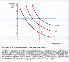
Curve showing all possible inputs with the same level of output. |
4 Production |
|
|
Marginal rate of technical substitution |
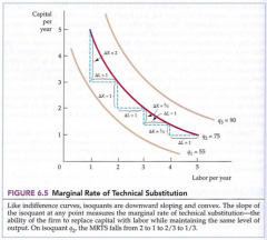
Amount by which the quantity of one input can be reduced when one extra unit of another input is used, so that output remains constant. (replace capital with labor while maintaining the same level of output.) MRTS= - Change in capital input/ change in labor input= - tlK/ flL (for a fixed level of q) |
4 Production |
|
|
Returns to scale |
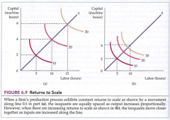
Rate at which output increases as inputs are increased proportionally. |
4 Production |
|
|
Constant returns to scale |
Situation in which output doubles when all inputs are doubled. f(2L, 2K) = 2f(L, K) |
4 Production |
|
|
Increasing returns to scale |
Situation in which output more than doubles when all inputs are doubled. f(2L, 2K) > 2f(L, K) |
4 Production |
|
|
Decreasing returns to scale |
Situation in which output less than doubles when all inputs are doubled. f(2L, 2K) < 2f(L, K) |
4 Production |
|
|
Accounting cost |
Actual expenses plus depreciation charges for capital equipment. |
4 Production |
|
|
Economic cost |
Cost to a firm of utilising economic resources in production, including opportunity cost. (statai namus ir tau kainuoja isvezt siuksles) |
4 Production |
|
|
Opportunity cost |
Cost associated with opportunities that are forgone when a firm when a firm's resources are not put to their best alternative use. (imone turi nuosava pastata ir puse jo yra nenaudojama, jie ji galetu nuomoti, taciau to nedaro ir taip praranda savo opportunity cost) |
4 Production |
|
|
Sunk costs |
Expenditure that has been made and cannot be recovered. (Because it has no alternative use, its opportunity costis zero.) (nusiperki equipment kuris gamina tik butelius ir pagamines butelius nebegali niekaip panaudot to equipment) |
4 Production |
|
|
Isocost line |
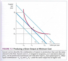
Graph of all possible combinations of labour and capital that can be purchased for a given total cost. C = wL + rK (cost = labour cost + capital cost) |
4 Production |