Reading...
![]()
Play button
![]()
Play button
![]()
Use LEFT and RIGHT arrow keys to navigate between flashcards;
Use UP and DOWN arrow keys to flip the card;
H to show hint;
A reads text to speech;
62 Cards in this Set
- Front
- Back
- 3rd side (hint)
|
Inflation
|
the overall increase in prices
|
|
|
|
Money
|
stock of assets that can be readily used to make transactions.
|
|
|
|
The function of Money
|
1. store of value, money is a way to transfer purchasing power from the present to the future.
2. unite of account, money provides the terms in which prices are quoted and debts are recorded. 3. Medium of exchange, money is what we use to buy goods and services. |
|
|
|
The types of Money
|
1. Fiat Money: money that has no intrinsic value is called fiat money because it is established as money by govt decree, or fiat.
2. Commodity money, money with intrinsi value. |
|
|
|
Money Supply
|
The quantity of money available in the economy.
|
|
|
|
Monetary Policy
|
The government's control over the money supply.
|
monetary policy (M)
fiscal policy (G;T) |
|
|
How to change money supply
|
1. open market operations: buy/sell govt bonds.
2. reserve requirement: ↑ the ratio that the bank keeps money so that Money SS ↓. 3. discount rate: bank's rate of borrowing money. ↑Discount rate ↑expense of banks ↓money SS. |
|
|
|
Quantity equation
|
M*V = P*T
money*velocity = price*transactions M*V = P*Y (Y, the total output of the economy, replaced T because transactions is difficult to measure) it holds by definition of the variables. |
1.Money: quantity of money
2. Velocity: tthe number of times a dollar bill changes hands in a given period of time. 3. Price: Price of a typical transaction, the number of dollars exchanged. 4. Transactions: tthe number of times in a year that goods or services are exchanged for money. 5. Y: real GDP 6. P: the GDP deflator 7. PY: nominal GDP |
|
|
Real Money Balance
|
M/P: measure the purchasing power of the stock of money.
(When we analyze how money affects the economy, it is often useful to express the quantity of money in terms of the quantity of goods and services it can buy.) |
|
|
|
Money Demand Function
|
an equation that shows the determinations of the quantity of real money balances people wish to hold.
(M/P )d = k Y k is a constant that tells how much money people want to hold for every dollar of income. |
1.This equation states that the quantity of real money balances demanded is proportional to real income.
2. (M/P)d = M/P so M/P = kY M(1/K)= PY Compared with MV = PY so: V= 1/k When people want to hold a lot of money for each dollar of income, money changes hands infrequently. |
|
|
Quantity theory of money
|
assumption of constant velocity, MV= PY. Therefore, M must cause a proportionate change in PY, in other words, quantity of money determines the dollar value of the economy's output.
|
|
|
|
a theory to explain what determines the economy's overall level of prices.
|
–With V constant, the money supply determines nominal
GDP (P*Y ). –Real GDP is determined by the economy’s supplies of K and L and the production function (Chap 3). –The price level is P = (nominal GDP)/(real GDP). |
%∆M+%∆V=%∆P+%∆Y
1. M under the control of central bank 2. V reflects shifts in money demand. zero here. 3. P rate of inflation 4. Y depends on growth in the factors of production and technological progress. So, the quantity theory of money states that the central bank has ultimate control over the rate of inflation. If the central bank increases the money supply rapidly, the price level will rise rapidly. |
|
|
Nominal Interest Rate
Real Interest Rate |
Nominal Interest Rate: the interest rate that the bank pays.
Real Interest Rate: the increase in purchasing power. r = i-π r= |
|
|
|
Fisher effect
|
i = r + π
Chap 3: S = I determines r . • Hence, an increase in causes an equal increase in i. • This one-for-one relationship is called the Fisher effect. |
According to quantity theory, an increase in the rate of money growth of 1 percent causes a 1 percent increase in the rate of inflation.
According to the Fisher equation, a 1 percent increase in the rate of inflation in turn causes a 1 percent increase in the nominal interest rate. |
|
|
Ex ante real interest rate
|
i – Eπ = ex ante real interest rate: the real interest rate people expect at the time they buy a bond or take out a loan.
|
|
|
|
Ex post real interest rate
|
i – π = ex post real interest rate: the real interest rate actually realized.
|
|
|
|
The (modified) money demand
function |
(M/P)d = L(i, Y)
The nominal interest rate is the opportunity cost of holding money: it is what you give up by holding money rather than bonds. The demand for real money balances depends both on the level of income and on the nominal interest rate. –negatively on i i is the opp. cost of holding money –positively on Y higher Y ⇒ more spending so, need more money |
M/P = L (r+eπ, Y)
1. M: exogenous (the Fed) 2. r: adjusts to ensure S = I 3. Y : Y= F (K, L) 4. P: adjusts to ensure M/P = L (i, Y) • For given values of r, Y, and Eπ , a change in M causes P to change by the same percentage – just like in the quantity theory of money. |
|
|
The costs of expected inflation
|
1. Shoeleather costs: the costs and inconveniences of reducing money balances to avoid the inflation tax.
2. Menu costs: costs of changing prices. 3. Relative price distortions: different firms change their prices at different times, leading to relative price distortions. 4. Unfair tax treatment: Some taxes are not adjusted to account for inflation, e.g. capital gains tax. 5. General inconvenience |
1. shoeleather costs: π ↑, i↑, (M/P)d ↓, k↓, people must more frequent trips to the bank to withdraw money--for example, they might withdraw $50 twice a week instead of $100 once a week.
2. Menu Cost: the higher the rate of inflation, the more often restaurants have to print new menus. 3. Relative price distortions: if inflation is 1%/ month, then at the end of the year, the firm's relative prices fall by 12%. Sales from this catalog will tend to be low in early but high later. Hence, when inflation induces variability in relative prices, it leads to microeconomic inefficiencies in the allocation of resources. 4. tax law 5. general inconvenience: to compare distances measured in different years, one would need to make an "inflation" correction. Similarly, the dollar is a less useful measure when its value is always changing. |
|
|
The costs of unexpected inflation
|
1. Additional cost of unexpected inflation: Arbitrary redistribution of purchasing power - Many long- term contracts not indexed, but based on Eπ . If π>eπ, debtor gains at the expense of the creditor because the debtor repays the loan with less valuable dollars.
2. Increased uncertainty: most people are risk avers, the unpredictability caused by highly variable inflation hurts almost everyone. |
|
|
|
One benefit of inflation
|
• Nominal wages are rarely reduced, even when the equilibrium real wage falls.
This hinders labor market clearing. • Inflation allows the real wages to reach equilibrium levels without nominal wage cuts. • Therefore, moderate inflation improves the functioning of labor markets. |
|
|
|
Hyperinflation
|
• Common definition: π ≥ 50% per month
• All the costs of moderate inflation described above become huge under hyperinflation. • Money ceases to function as a store of value, and may not serve its other functions (unit of account, medium of exchange). • People may conduct transactions with barter or a stable foreign currency. |
|
|
|
The Cause of Hyperinflation
|
1. begin when the government has inadequate tax revenue to pay for its spending.
2. govt might issue debt but find itself unable to borrow bc of bad credit risk. 3. turns to the only mechanism--the printing press. |
once the hyperinflation is under way, the fiscal problems become more severe. Because of the delay in collecting tax, real tax revenue falls as inflation rises. Thus, govt need to rely self-reinforcing. Rapid money creation leads to hyperinflation, which leads to a larger budget deficit, which leads to even more rapid money creation.
|
|
|
The End of Hyperinflation
|
The ends almost always coincide with fiscal reforms. The govt musters the political will to reduce govt spending and increase taxes. These fiscal reforms reduce the need for seigniorage, which allows a reduction in money growth. Hence, even if inflation is a monetary phenomenon, the end of hyperinflation is often a fiscal phenomenon as well.
|
|
|
|
The Classical Dichotomy
|
The theoretical separation of real and nominal variables.
**Real variables: Measured in physical units, for example: –quantity of output produced –w/p: output earned per hour of work –r: output earned in the future by lending one unit of output today **Nominal variables: Measured in money units, e.g., -W: Dollars per hour of work. -I: Dollars earned in future by lending one dollar today. -P: The amount of dollars needed to buy a representative basket of goods. |
The classical dichotomy arises because, in classical economic theory, changes in the money supply do not influence real variables. This irrelevance of money for real variables is called monetary neutrality.
|
|
|
Neutrality of money
|
Changes in the money
supply do not affect real variables. In the real world, money is approximately neutral in the long run. |
|
|
|
Natural Rate of Unemployment
|
The average rate of unemployment around which the economy fluctuates.
|
|
|
|
Frictional Unemployment
|
The unemployment caused by the time it takes workers to search for a job.
|
|
|
|
Cause of Frictional Unemployment
|
1. imperfect information flows
2. geographic mobility 3. different skills, abilities and preference 4. different job requirement 5. sectoral shift |
|
|
|
Sectoral Shift
|
Changes in the composition of demand among industries or regions.
|
1.Examples: technological change, a new international trade agreement.
2. different from recession, overall demand did not change. |
|
|
Public Policy to Solve Frictional Unemployment
|
1.Govt employment agencies
2.Public job training programs 3.Crete Job 4. Unemployment Insurance |
Unemployment insurance (UI):
•UI increases frictional unemployment by reducing the opportunity cost of being employed and the urgency of finding work. • By allowing workers more search time, UI may lead to better matches between jobs and workers, thus increasing productivity and incomes. |
|
|
Wage Rigidity
|
The failure of wage to adjust to a level at which labor supply equals labor demand.
|
|
|
|
Reasons for Wage Rigidity
|
1.Minimum wage laws: The min. wage may exceed the eq’m wage of unskilled workers, especially teenagers, resulting in unemployment.
2.Labor unions: unions exercise monopoly power to secure higher wages for their members. When the union wage exceeds the eq’m wage, unemployment results. 3.Efficiency wages: Firms willingly pay workers wages above equilibrium to increase workers’ productivity, resulting in structural unemployment. |
1. Minimum Wage Law: reduce poverty and provide relief but poor targeted.
2. Labor Union: outsider may become the one who loses job. 3. Adverse selection (the tendency of people with more information to self-select in a way that disadvantages people with less information); Moral Hazard. |
|
|
Structural Unemployment
|
The unemployment resulting from wage rigidity and job rationing.
|
|
|
|
Duration of Unemployment
|
1.More spells of unemployment are short-term than medium-term or long-term. (number)
2. most of the total time spent unemployed is attributable to the long-term unemployed.(duration) |
|
|
|
Facts about the business cycle
|
1.GDP growth averages 3–3.5 percent per year over the long run with large fluctuations in the short run.
2.Consumption and investment fluctuate with GDP, but investment is more volatile than consumption. 3.consumption and investment spending decline while unemployment rises in recession. 4.Okun's Law |
|
|
|
Okun's Law
|
1.the negative relationship between GDP and unemployment.
2.Percentage change in real GDP = 3%-2*Change in the Unemployment rate |
|
|
|
Business Cycle Announcement and Forecasting
|
1.NBER’s Business Cycle Dating Committee: official arbiter of the beginning and end of recessions.
2.Index of Leading Economic Indicators: published monthly by the Conference Board. - Aims to forecast changes in economic activity 6-9 months into the future. - Used in planning by businesses and govt, despite not being a perfect predictor. |
|
|
|
Leading Indicators
|
variables that tend to fluctuate in advance of the overall economy.
|
1. Average workweek of Production workers in manufacturing.
2. Average initial weekly claims for unemployment insurance. 3. New orders for consumer goods and materials, adjusted for inflation. 4. INdex of suppler deliveries (Vendor Performance). 5. New building permits issued. 6. Index of stock prices. 7. Money supply (M2), adjusted for inflation. 8. Interest rate spread: the yield spread between 10-year Treasury notes and 3-monts Treasury bills. 9. Index of consumer expectations. |
|
|
The difference between LR and SR
|
In LR price are flexible, respond to changes in supply or demand while in SR many price are sticky at predetermined level.
|
|
|
|
Aggregate Demand
|
Relationship between the quantity of output demanded and the aggregate price level.
|
1. tells us the quantity of goods and services ppl want to buy at any given level of prices.
2. sloping downward. 3. AD is drawn for a fixed value of money supply. |
|
|
Why the AD downward-sloping?
|
An increase in the price level causes a fall in real money balances (M/P), causing a decrease in the demand for goods & services.
|
P270 three types of explain
|
|
|
The shift of AD
|
An increase in the money supply shifts the AD curve to the right.
|
An increase in the M raises the nominal value of output PY. For any given price level P, output Y is higher.
|
|
|
Aggregate Supply
|
the relationship between the quantity of goods and services supplied and the price level.
|
because the firms that supply goods and services have flexible P in LR but sticky P in SR, the AS depends on the time horizon.
|
|
|
LRAS
|
the level of output is determined by the K and L and available technology; does not depend on P. LRAS is vertical
|
In the long run, this raises the price level but
leaves output constant. |
|
|
SRAS
|
all prices are fixed in SR so the SRAS is horizontal;firms sell as much as buyers demand.
|
1. In the short run when prices are sticky, an increase in M causes output to increase.
2. After the sudden fall in AD, firms are stuck with prices that are too high. With demand low and price high, firms sell less of their product, so they reduce production and lay off workers. The economy experiences a recession. |
|
|
From SR to LR (a reduction in AD)
|
In SR, P sticky so the economy moves from A to B, where Y decreases, output and employment fall below natural levels, which means the economy is in a recession. Over time, in response to the low demand, wages and prices fall. The gradual reduction in P moves the economy downward along the AD curve to point C, which is the new LR equilibrium. In C, output and employment are back to their natural levels, but P are lower than A.
Thus, a shift in AD affects output in RS but this effect dissipates over time as firms adjust their prices. |
|
|
|
Shock
|
1. Exogenous changes in aggregate supply or demand.
2.Shock disrupt the economy by pushing output and employment away from their natural levels. |
Example: exogenous decrease in velocity
If the money supply is held constant, a decrease in V means people will be using their money in fewer transactions, causing a decrease in demand for goods and services. |
|
|
Demand Shock
|
A shock that shifts the AD curve.
|
Example: the introduction of credit cards. Holding less money, the money demand parameter k falls, velocity rises. AD moves outwards.
|
|
|
Supply Shock
|
A supply shock alters production costs, affects the prices that firms charge. (also called price shocks)
|
Examples of adverse supply shocks: – Bad weather reduces crop yields, pushing up
food prices. – Workers unionize, negotiate wage increases. – New environmental regulations require firms to reduce emissions. Firms charge higher prices to help cover the costs of compliance. Favorable supply shocks lower costs and prices. |
|
|
Stagflation
|
A combination of increasing prices and falling output.
|
|
|
|
Stabilization Policy
|
Policy actions aimed at reducing the severity of short-run economic fluctuations.
|
Example: Using monetary policy to combat the effects of Adverse supply shocks
The adverse supply shock pushes up costs and thus prices, moving SRAS upwards, leading to stagflation--a combination of increasing P and falling Y. But the Fed accommodates the shock by raising agg. demand. RESULT: P is permanently higher, but Y remains at its full- employment level. |
|
|
The Keynesian Cross
|
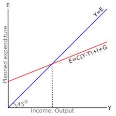
A simple closed economy model in which income is determined by expenditure.
equilibrium condition: actual expenditure = planned expenditure Y (AE) = PE |
I = planned investment
PE = C + I + G = planned expenditure Y = real GDP = actual expenditure |
|
|
An increase in government purchases--Government Purchases multiplier
|
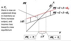
At Y1, there is now an unplanned drop in inventory so firms increase output, and income rises toward a new equilibrium.
∆Y/∆G = 1/(1-MPC) |
prove of government purchases multiplier:
Y = C+I+G eq'm condition ∆Y=∆C+∆I+∆G =∆C+∆G =MPC*∆Y+∆G So, (1-MPC)*∆Y=∆G |
|
|
An increase in tax in Keynesian cross--Tax Multiplier
|
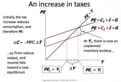
The tax increase reduces consumption. At Y1, there is now an unplanned inventory buildup. So firms reduce output, and income falls toward a new equilibrium.
Tax multiplier: ∆Y/∆T = - MPC/ (1-MPC) |
prove of tax multiplier:
∆Y = ∆C+∆I+∆G = ∆C = MPC (∆Y-∆T) Solving for ∆Y |
|
|
IS curve
|
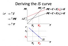
a graph of all combinations of r and Y that result in goods market equilibrium : actual expenditure (output) = planned expenditure
The equation for the IS curve is: Y = C(Y-T) + I(r) + G |
Why the IS curve is negatively sloped?
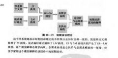
• A fall in the interest rate motivates firms to increase investment spending, which drives up total planned spending (PE ). • To restore equilibrium in the goods market, output (i.e., actual expenditure, Y ) must increase. IS曲线结合了投资函数表示的r和I之间的相互作用和凯恩斯交叉图表示的I和Y之间的相互作用。IS曲线的每一点都代表产品市场上均衡,该曲线显示了均衡收入水平如何依赖于利率。 |
|
|
How fiscal policy shifts the IS curve
|
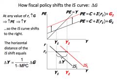
IS曲线表示产品和服务市场均衡一致的利率与收入水平的结合。
|
|
|
|
Theory of Liquidity Preference
|
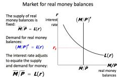
A simple theory in which the interest rate is determined by money supply and money demand.
|
流动偏好理论假定,利率调节使经济中最具流动性的资产-货币-供求平衡;而凯恩斯交叉图说明了家庭、企业和政府的支出计划如何决定国民收入。
|
|
|
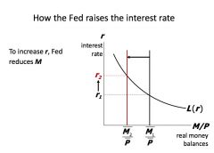
How does the interest rate adjust money supply and demand into equilibrium (if M changes)?
|
XXXXX
|
|
|
|
LM curve
|
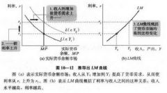
a graph of all combinations of r and Y that equate the supply and demand for real money balances.
Equation for LM: M/P = L (r, Y) |
LM曲线上的每一点都代表货币市场的均衡,曲线表示均衡利率如何依赖于收入水平。收入水平越高,实际货币需求越高,利率也越高。由于这个原因,LM曲线向右上方倾斜。
Why the LM curve is upward sloping • An increase in income raises money demand. • Since the supply of real balances is fixed, there is now excess demand in the money market at the initial interest rate. • The interest rate must rise to restore equilibrium in the money market. |
|
|
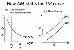
How monetary policy shift LM curves (∆M)?
|
XXXX
|
LM曲线表示与实际货币余额市场的均衡相一致的利率和收入水平的结合。LM曲线是根据一个给定的实际货币余额的供给绘制的。实际货币余额供给的减少使LM曲线向上移动。实际货币余额供给的增加使LM曲线向下移动。
|
|
|
The short-run equilibrium (Chapter 10)
|
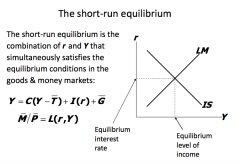
The short-run equilibrium is the combination of r and Y that simultaneously satisfies the equilibrium conditions in the goods & money markets.
Equilibrium is where IS curve cross LM curve. At this point, AE=PE, (M/P)ss=(M/P)dd |
|
|
|
The role of Short Run equilibrium
|
|
|