![]()
![]()
![]()
Use LEFT and RIGHT arrow keys to navigate between flashcards;
Use UP and DOWN arrow keys to flip the card;
H to show hint;
A reads text to speech;
34 Cards in this Set
- Front
- Back
|
Injective |
If f(x) = f(y) x=y (outputs can only hv1 input) |
|
|
Surjective |
If our codomaine is B and y is in B then there exists some x where f(x) = y (all y have an x) |
|
|
Image of a linear map |
The set of outputs |
|
|
Kernel |
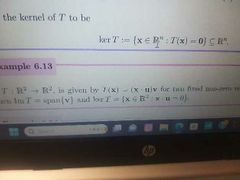
The inputs that map to 0 |
|
|
Nullity T |
Dim ker T |
|
|
Rank |
Dim Im T |
|
|
Rank nullity theorem |
Dim(T) = rankT + nullityT |
|
|
Fundamental theorem of algebra |
every polynomial equation of degree n with complex number coefficients has n roots, or solutions, in the complex numbers |
|
|
Isomophism |
Linear map thats bijective (a map that preserves the desired structure) |
|
|
If V and W are vector spaces (both over a field K) of the same dimension n then V and W are
|
isomorphic
|
|
|
Let V , W be two vector spaces over the same field K. Then a function f : V → W is called a linear map if for all a, b ∈ K and u, v ∈ V
|
f(au + bv) = af(u) + bf(v).
|
|
|
Theorem 1.28. Let V /= {0} be a vector space and we assume that there exists a finite set S which spans V . Then
|
(1) There exists a subset of S which is a basis for V . In particular, V is finite-dimensional. (2) If a subset T ⊂ V is linearly independent then T can be extended to a basis of V . (3) If U is a subspace of V then U is finite-dimensional. If furthermore dim U = dim V then U = V
|
|
|
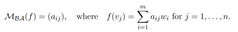
Definition 1.30 (Matrix of a linear map). Let V, W be vector spaces over a field K. Let A = {v1, . . . , vn} be an ordered basis of V and B = {w1, . . . , wm} an ordered basis of W. Given f ∈ L(V, W), the matrix associated to f (with respect to the bases A, B) is the m × n matrix
|
|
|
|
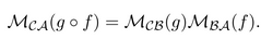
Let U, V, W be vector spaces over a field K with ordered bases A = {u1, . . . , ul}, B ={v1, . . . , vm} and C = {w1, . . . , wn}, respectively and suppose f : U → V and g : V → W are linear maps.Let MBA(f) = (aij ) be the matrix of f and MCB(g) = (bij ) the matrix of g relative to these bases. Theng ◦ f : U → W has matrix |
|
|
|
Definition 1.37. Matrices A and A' are said to be similar, denoted A ~A' |
if there exists an invertible matrix C such that A' = C −1AC. Similarity defines an equivalence relation on the space of square n × n matrices |
|
|
Theorem 1.38. Suppose that A~ A' and A represents a linear operator f relative to some ordered basisB = {v1, . . . , vn}. |
Then there is an ordered basis B' = {v' 1 , . . . , v'n} relative to which f has matrix A; |
|
|
Let A, B ∈be Mn(K) be similar matrices. Then pA(x) |
= pB(x). |
|
|
Lemma 1.44. Let A ∈be Mn(K). Then the constant coefficient of pA(x) equals |
det(A). |
|
|
if A is similar to B, then det(A) = |
det(B). |
|
|
Definition 1.45. Let A be Mn(K). Then the trace of A, denoted trA, is equal to = |
Sum of aii |
|
|
Lemma 1.46. Let A be Mn(K). Then the x^n−1coefficient of pA(x) equals |
(−1)^n−1 tr(A). |
|
|
A is similar to B, then tr(A) = |
tr(B) |
|
|
Definition 1.1. A function f : Rn → Rm is called R-linear if it satisfies two properties:
|
• f(v + w) = f(v) + f(w) for all v, w ∈ Rn; and • f(λv) = λf(v) for all v ∈ Rn and λ ∈ R.
|
|
|
Definition 1.2. A function f : C n → C m is called C-linear if it satisfies two properties:
|
• f(v + w) = f(v) + f(w) for all v, w ∈ C n; and • f(λv) = λf(v) for all v ∈ C n and λ ∈ C.
|
|
|
Definition 1.3. Let V and W be vector spaces (technically over a field F). Then a function f : V → W is called F-linear if it satisfies two properties:
|
• f(v + w) = f(v) + f(w) for all v, w ∈ V ; and • f(λv) = λf(v) for all v ∈ V and λ ∈ F. If, from the context, the field F is clear, then we will talk about the function f being linear and omit the notation of F.
|
|
|
Definition 1.7. Fix an n ∈ {1, 2, 3, . . .} and choose an i ∈ {1, . . . , n}. Then ei
|
is the vector in Rn with ith entry 1 and all other entries zero. Another way to phrase this is that the jth entry of ei is given by the Kronecker delta function δij .
|
|
|
Lemma 1.10. Let V and W be vector spaces over F and f and g be F-linear functions from V to W such that f(ei) = g(ei) for all valid i. Then
|
f = g
|
|
|
Definition 2.1. Let V be a vector space over F and T : V → V a linear operator. Then a vector v ∈ V with v /=0 is called an eigenvector of T if
|
there exists a λ ∈ F such that T(v) = λv . The number λ is the called an eigenvalue of T.
|
|
|
Definition 2.4. Let T : V → V be a linear operator, we call the set of eigenvalues of T
|
the spectrum of T, denoted spec T.
|
|
|
Lemma 2.5. Let T : V → V be a linear operator and λ be an eigenvalue for T. Then the set of eigenvectors for λ, together with the zero vector,
|
form a subspace of V
|
|
|
Theorem 2.6. Let T : V → V be a linear operator and dim V < ∞. Then λ ∈ F is an eigenvalue of T if and only if
|
det(T − λI) = 0.
|
|
|
Definition 2.7. Let V be vector space over F and T : V → V be a linear operator,
|
• if dim V < ∞ then the characteristic polynomial of T is defined as pT (x) := det(T − xI). • if λ ∈ F is an eigenvalue of T the corresponding eigenspace is defined as E(λ) := ker(T − λI)
|
|
|
Definition 2.17. For a polynomial p(x) we say that λ1 ∈ C is a root of p if
|
p(λ1) = 0.
|
|
|
We can also talk about the multiplicity of a root. Specifically, if λ1 is a root of multiplicity m1
|
there exists a polynomial q(x) of degree n-m1 with q(λ1) /= 0 where p(x) = (x − λ1) m1 q(x), Note that the multiplicity of any root is a natural number.
|