![]()
![]()
![]()
Use LEFT and RIGHT arrow keys to navigate between flashcards;
Use UP and DOWN arrow keys to flip the card;
H to show hint;
A reads text to speech;
12 Cards in this Set
- Front
- Back
- 3rd side (hint)
|
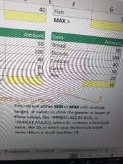
Explain min max functions. |
|
|
|
|
Hdhdhd |
Rhfhhffh |
|
|
|
Rhdhdh |
Thfhfhhf |
|
|
|
Join text from different cells. |
In new cell use formula =c3&d3 You can also add spaces commas etc. By using qoutes example &" "&. =c3&" "&d3 |
It like summing two cells with numbers but you use & sign for text. |
|
|
Give an example of an IF statement. |
=IF(C9="Apple",TRUE,FALSE)
|
=IF(C12<100,"less than 100","Greater than or equal to 100") Numbers and TRUE and FALSE dont need to be in quotes. |
|
|
IF statement w another function |
=IF(E33="YES", F31*SalesTax,0) |
If cell is yes than multiply othercell by SalesTax if otherwise show 0. |
|
|
Give example of named ranges and how you can create them or acces them. |
Named range can be accessed from Formulas > Name Manager Example you can set sales=2.4% |
Its basically a constant. Or a text serving as a number. SalesTax is a number and thus doesnt need quotes in a formula. |
|
|
Explain =VLOOKUP(A1,B:C,2,FALSE) |
A1 = search bar cell. B:C = the whole table. 2 = the second column where the desired value is to be extracted from FALSE= Exact match. |
Its a search bar. |
|
|
(#N/A) created when refernce value doesn't exist in cell. Or the lookup doesnt exist. Whats one way of fixing it |
=IF(C43="","",VLOOKUP(C43,C47:D41,2,FALSE)) Essentially if there is no entry in C43..."" show "". |
If there is nothing... indicated by "" than show "" instead of #N/A. |
|
|
Define Conditional functions- "SUMIF" |
Conditional functions lets you sum,avg,count, get min or max of a range based on a given condition or criteria. |
|
|
|
Explain =SUMIFS(H3:H14, F3:F14,F17 ,G3:G14,G17) |
H3:H14= The range you want to sum F3:F14,F17= First range to look in for matches, F17 is the criteria G3:G14,G17= Second range to look in for matches,G17 is the criteria for second match. |
You want to sum Amount based on Fruit AND Type shown. |
|
|
Explain =SUMIF(C3:C14,C17, D3:D4) |
C3:C14=The range you need to look at C17=value to look for apples oranges bananas.... D3:D14=range of values to sum up. |
|