Set the Language

We weren't able to detect the audio language on your flashcards. Please select the correct language below.

Front

Back

Related Flashcards

Flashcards
»
Microeconomics

Microeconomics

by joeprince9, Feb. 2016

Subjects: Microeconomics

Favorite

Add to folder

Flag

Shuffle
Toggle On

Toggle Off
Alphabetize
Toggle On

Toggle Off
Front First
Toggle On

Toggle Off
Both Sides
Toggle On

Toggle Off
Read
Toggle On

Toggle Off

Reading...

Front

Card Range To Study

through

Play button

Progress

1/96

Click to flip

Use LEFT and RIGHT arrow keys to navigate between flashcards;

Use UP and DOWN arrow keys to flip the card;

H to show hint;

A reads text to speech;

96 Cards in this Set

Front
Back

	What is a pure strategy?	A pure strategy is a plan of action. - A complete specification of what a play should do whenever that player has to make a choice - Allows history-dependence, i.e. it can condition how you play on the other players' earlier actions in the game - It does not permit randomisation
	What is a mixed strategy?	A mixed strategy allows players to randomise - It specifies a probability with which each pure strategy is to be selected
	What is a strategy profile? What does s⁃ᵢ denote?	A strategy profile (s₁, s₂, ... sn) is a list identifying a particular strategy for every player in the game (of N players in this case). - It is essentially a list of everybody's strategies. s⁃ᵢ is the strategy profile for every player except for player i
	What is a payoff function uᵢ (sᵢ, s⁃ᵢ)? What is a best response? / How would player i calculate their best response s*ᵢ in this format?	uᵢ (sᵢ, s⁃ᵢ) tells us what player i's payoff will be given what everyone else does, and what player i does. Player i's best response is a sᵢ is a strategy which maximises her own payoff. It must be at provide a payoff which is at least as good as any other payoff, i.e. uᵢ (sᵢ,** s⁃ᵢ) ≥ uᵢ (sᵢ, s⁃ᵢ)
	What is a dominant strategy?	A dominant strategy is a best response to every possible strategy profile for the other players. - So whatever the other players do, the dominant strategy maximises player i's payoff - If this exists for a player, the player will always employ the strategy - But in most games, players will not have dominant strategies
	When do pure strategies and actions coincide?	Pure strategies and actions coincide in a one-shot game, i.e. in a game when players take just one action. In general, this is not the case, since straggles specify the actions that a player would take for every possible eventuality.
	What is a Nash Equilibrium? What is it formally (notationally)? What is the Equilibrium outcome?	A Nash Equilibrium (NE) is a set of strategies (one for each player) such that each player's strategy is a best response to the strategies of the other players. - At a Nash equilibrium, no player wants to change her strategy (given what the other plays are doing) - Some games have more than one Nash Equilibrium Formally: NE is a set of strategies, {s₁, s₂...sɴ) suchh that for every player i, uᵢ (sᵢ, s⁃ᵢ) ≥ uᵢ (sᵢ, s⁃ᵢ) The equilibrium outcome is the set of actions and payoffs which results from the Nash Equilibrium strategies being played.
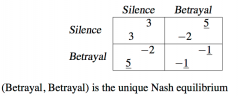
	What is a dominant strategy equilibrium?	A dominant strategy equilibrium will occur when each player has a dominant strategy (which they will employ no matter what, since ti will always be their best response given what their opponent is doing). So, each player choosing Betrayal must be a rest response to the other player doing the same.
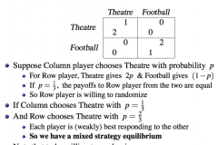
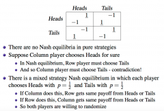
	What is a mixed strategy equilibrium? When should we look for a mixed strategy equilibrium?	A mixed strategy equilibrium occurs when each player is willing to randomise. To be willing to randomise, a player has to be exactly indifferent between the strategies. If this is the case, then act player will be rest responding to the other. We should always look for a mixed strategy equilibrium, since this is a possible action that a player could take (if it yields the same or greater expected payoff than the pure strategy). - We should especially look for a mixed strategy if at least one player does not have strictly dominant strategies - but if all players have strictly dominant strategies, then they want ever wish to do anything else
	If there are no Nash Equilibria in pure strategies, can there still be a mixed strategy equilibrium?	Yes
	Is Nash Equilibrium sensible? (Yes vs No)	Yes: - If players do not play Nash Equilibrium ex post they would feel they had made the wrong choice No: - Agents are not necessarily rational, and cannot always predict how others will play But: - Agents can 'learn' to play Nash Equilibrium with experience - They learn to predict better how others will play - They learn how to best responds
	What is Cournot Competition? What is Bertrand Competition? What is Stackelberg Competition?	Cournot Competition: - Firms choose quantities (simultaneously), and the market determines prices - A cournot "auctioneer" adjusts prices so that the market clears - e.g. hotel rooms Bertrand Competition: - Firms choose prices (simultaneously), and the market determines the quantities demanded for each firm - e.g. supermarket products Stackelberg Competition: - Same as Cournot, where firms choose quantities, but with sequential moves - There is a leader that chooses first and a follower that sees the leader's choice before choosing her output - The follower's output (given any leader's output) is the same as in Cournot - But the leader can anticipate this response, and so chooses quantity to maximise his own profits, i.e. max π₁ (q₁, q*₂(q₁))
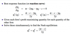
	How would you find the best response function (or reaction curve) in Cournot competition?	Partially differentiate profits of each firm (which depend on the quantity of the other firm) with respect to their own quantity, i.e. taking the other quantity as a given. Solve these simultaneously to find the Cournot-Nash Equilibrium - At this point, each firm's quantity choice is a best response to the other firm's quantity - Profits and prices are higher than in competitive markets, but lower than in monopoly
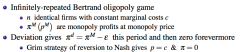
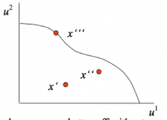
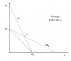
	What does the graph of Cournot-Nash equilibrium look like and the best-response functions under Cournot competition? Why are the best-response functions downward sloping?	Downward sloping because: - The more the other produces (which you are taking as a given), then less residual demand there would be for you - so the less you would produce yourself. - Quantities are strategic substitutes
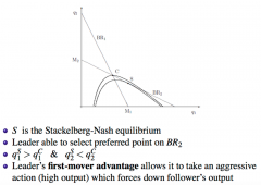
	What does the graph of Stackelberg-Nash Equilibrium look like and the best-response functions under Stackelberg competition?	- Best Response Functions are the same as Cournot - Leader can choose any point along BR₂ (what his opponent will choose) that is preferred most for him (where his own profit is maximised, as shown here by isoprofit lines) - The equilibrium is more aggressive (for the leader) than in Cournot, since it forces down the follower's output
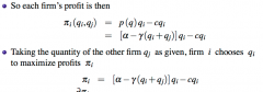
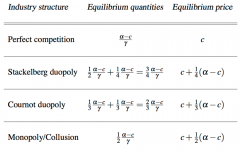
	If firms have a constant marginal cost c, have no fixed costs, and face the demand curve p = α - ɣ(qᵢ+qj) , then compare the possible output/price outcomes for perfect competition, stackelberg duopoly, cournot duopoly, and monopoly/collusion	So total equilibrium quantity gets smaller as we move toward monopoly, and the equilibrium price gets larger.
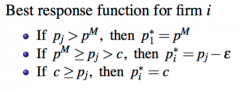
	What is the best-response function for firm i under Bertrand competition in a duopoly? What are the Bertrand competition assumptions to derive these response functions?	Assumptions: - Firms choose prices simultaneous - Consumers buy from the lowest price firm (since products are homogeneous) - So if firm 1 undercuts firm 2, then q₁ = p(q₁) and q₂ = 0, i.e. only his quantity determines the market price, since no one is buying from firm 2 - If their prices are equal, then they split the market, i.e. q₁ = q₂ = q(pᵢ) / 2
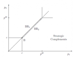
	What does the graph of Bertrand-Nash equilibrium look like and best-response functions under Bertrand competition? What is the unique Bertrand-nash equilibrium and why? Why is the Best-Response function upward sloping?	Unique Bertrand-Nash equilibrium is where both firms price at marginal cost - Best response functions intersect at pᵢ = pj = c - So in equilibrium, both firms price at marginal cost - We cannot have an equilibrium with higher prices, as the higher price firm would always want to undercut the lower price firm The best-response function is upward-sloping because: - the higher the rival price, the higher the price that I want to set - Prices are strategic complements
	What is the Bertrand paradox? Why is this a knife-edge result?	It seems paradoxical for competition between just two firms to lead to marginal cost pricing Prices and quantities look like those in competitive markets, and firms make zero profits. The Bertrand Paradox is a knife-edge result since it depends on the fact that the products are identical. - Since with differentiation, Bertrand profits and prices are higher than in competitive markets (but lower than monopoly) and total quantity is lower than in competitive markets (but higher than monopoly)
	What is the difference between vertical product differentiation and horizontal product differentiation?	Vertical Differentiation: - Goods vary in quality - If the goods sell at the same price, everybody chooses the higher quality variety - e.g. Medical Care Horizontal Differentiations: - Goods vary on dimensions other than quality - If the goods are the same, then consumers differ in their ranking - e.g. Breakfast Cereals (different in taste, which is subjective)
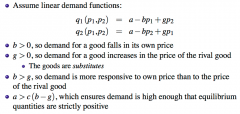
	Describe the model of Bertrand competition with differentiated products? How would you find the Nash Equilibrium? Are the best-response functions positively or negatively sloped? Why?	Two firms produce horizontally differentiated product - so they are no longer identical/homogenous - But they are imperfect substitutes for each other (e.g. Honda and Volkswagen) Nash Equilibrium: - Find each firm's profit function - Taking the price of the other firm as given, firm i choose its own price to maximise its profits - Obtain the FOCs to find their best response functions, giving each firm's profit maximise prince for each price of the other firm - Solve these simultaneously to find the Nash Equilibrium Best response functions are positively sloped! - As the other firm raises its price, it is less competitive - So I can raise my price
	What is extensive form in game theory?	Decision tree diagram showing payoffs.
	What is a subgame perfect equilibrium?	A subgame perfect equilibrium is a type of Nash Equilibrium - ...if the players' strategies constitute a Nash Equilibrium in every subgame SPE rules out incredible threats, which can exist in a Nash Equilibrium
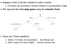
	What can an incumbent do to deter entry if its threat to fight the incumbent upon entry is not credible?	It could take pre-emptive action to deter entry - e.g. If entrant, had to pay a fixed cost F to enter, then the incumbent can commit to an action which refuels entrant profits below F - e.g. can pre-emptively increase its capital Kᵢ (a sunk cost) to reduce its marginal cost, and hence commits it to being more aggressive, i.e. producing more itself and reducing other's profits - This would cause its best response curve pushed out to the right (raising his own quantity, lowing the entrant's quantity, and lowering the entrant's profits) - This commitment makes the threat credible If this is too expensive, then the entry will be accommodated
	What is the Backward induction?	When the game is finite, find the subgame perfect equilibria by working backwards from the later sub-games - Find the Nash Equilibria of the later subgames - Given these, find the equilibria of the earlier subgames - Continue all the way back until the beginning of the game tree, i.e. unravelling the game
	What is the sub-game perfect equilibria in finitely repeated games with? More generally, what is the Sub-game perfect equilibrium of a finitely repeatedly game with a unique Nash Equilibrium?	Backward Induction: - The final subgame is just like that in the one-shot prisoners' dilemma, so both prisoners will betray (whatever the history, this is a dominant strategy) - Knowing that they will both betray in the last period they will also both betray in the second-last period as well - And hence they will both betray in the third-last period and so on... In general, if a stage game with a unique Nash Equilibrium is played a fixed and finite number of times, the unique Sub-game perfect equilibrium of the repeated game is to play the stage game Nash Equilibrium in every period - This is what makes collusion impossible in the finitely repeated Cournot Game (assuming that firms always play SPE), i.e. threats of punishment for not cooperating are incredible
	What is a Trigger Strategy? What is a Grim Trigger Strategy?	Trigger: - Play X as long as opponent doesn't play Y, in which case play Z (which can be the same as Y) Grim Trigger: - Once play of Z is triggered, continue playing Z forever
	Describe the Collusion Model in Cournot Duopoly, where a Grim-trigger strategy is employed by each firm? (It is an infinitely repeated game) When can these grim trigger strategies produce a subgame perfect equilibrium?	The firms attempt to collude to jointly produce the monopoly quantity qᴹ. Grim-trigger strategy for each firm: - In the first period, produce qᵢ = qᴹ/2 - In later periods, continue to produce qᵢ = qᴹ/2 as long as both firms have done so in every period up to that point - If either firm ever deviates from qᴹ/2, then produce Cournot-Nash equilibrium quantity qc forevermore --> i.e. the firms collude unless a firm deviates, in which case, they revert to the (less profitable) stage game Cournot-Nash equilibrium Playing the grim-trigger strategy gives πᴹ/2 in every period - The discounted value is πᴹ/2 + δπᴹ/2 + δ²πᴹ/2 + ... = (1/1-δ).πᴹ/2 Deviating gives profit πᵈ this period and then the Cournot-nash profit πc forevermore - The discounted value is πᵈ + (δ/1-δ)πc So firms will stick to the grim-trigger strategy if: (1/1-δ).πᴹ/2 > πᵈ + (δ/1-δ)πc Rearranging gives: δ > (πᵈ - πᴹ/2) / ((πᵈ - πc) So, strategies are sub-game perfect is firms are sufficiently patient. - i.e. if they don't discount the future too much (sufficiently high δ), then the one-period gain from deviating is outweighed by the reversion to Cournot-Nash equilibrium forevermore
	What does it mean for a payoff pair (i.e., one for each person) to be feasible?	A payoff pair is feasible if there is a pair of strategies that generates it.
	What is a minimax punishment? What is the minimax payoff?	A minimax punishment is the worst that one player can do to the other, given that the other is responding optimally. - e.g. if firm 1's quantity q₁ minimaxes firm 2 if it is chosen to minimise maxq₂ {π₂ (q₁, q₂) } When firm 2 responds optimally to being minimax punished, it receives the minimax payoff. A strategy is individually rational for a player if it guarantees that players at least his minimax payoff
	What is the Folk Theorem?	Folk Theorem: Any feasible payoff pairs which gives each player at least her minimax payoff can be supported as a Nash equilibrium in an infinitely repeated game if the discount factor δ is sufficiently close to 1. - So trigger strategies used to sustain equilibrium will use minimax punishments
	What is a horizontal agreement? Give examples	A horizontal agreement is one between firms at the same level in the industry. Examples: - price fixing - quantity fixing - explicit collusion - collusive tendering - market sharing - information agreements Also: - "Concerted Practice", i.e. tacit collusion (when there is no formal agreement in place)
	What factors affect the likelihood of collusion?	- Number of firms - Real interest rate - Frequency of Sales - Ease of Detecting Cheating - Coordination difficulties - Leniency programmes
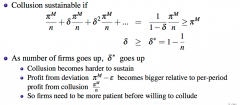
	Given this model, show why firms need to be more patient if they are willing to collude in a market with a larger number of firms? Why is this true intuitively? So ceteris paribus, does more firms make collusion more or less likely?	Note: we can ignore ε in the analysis because it is arbitrarily small Intuitively: - Collusion between more firms means getting a smaller share of the profit - This means the profit from deviation looks more attractive relative to the collusion profit - So firms must be sufficiently patient (care enough about future income enough) to sustain the collusion instead of deviating So more firms makes collusion less likely - for a given level of patience, more firms means I am more likely to be not patient enough to meet the new threshold of patience
	How does the interest rest affect the likelihood of collusion?	The discount factor is defined as δ = 1/(1+r) - So the higher the discount/real interest rate r, the more you discount future profits. - So the higher the real interest rate, the less weight we put on future profits - This means firms are less patient - This means firms are more willing to deviate to capture the monopoly profit sooner instead of sustaining the collusion profit - Therefore a higher interest rate makes collusion less likely - Also, since discounting the future more also means that the punishment is further in the future too, so we care less about that and would want to deviate now!
	How does the frequency of sales affect the likelihood of collusion? Give an example of infrequent sales.	If goods are sold less frequently: - Each later 'period' in which you earn the collusion profit is further in the future - For any δ < 1, this means we discount these periods even more (or our discount factor decreases further...) - Therefore, the less frequent the sales, the less weight we put on future profits - This means firms are less patient - This means firms are more willing to deviate to capture the monopoly profit sooner instead of sustaining the collusion profit - Therefore less frequent sales makes collusion less likely Example: Airplane Manufacturers - Orders don't happen everyday - So prices are only changed every few months - Punishment is further away, and we are not patient enough to obtain collusion profits every year, so are more likely to deviate, and less likely to collude.
	How does the ease of detecting cheating affect the likelihood of collusion? When is it easier to detect cheating?	Collusion is more likely to occur the easier it is to detect cheating (since firms will be less likely to deviate from any agreement) It is easier to detect cheating when: - price transparency: if prices are public information, then any deviation will be more evident to everyone who can see these prices - price matching guarantees: e.g. John Lewis: "never knowingly undersold" slogan means that (if it were in a collusive agreement) it spends time researching to see if other firms deviate, and this commits it to a credible threat of retaliation. - Demand uncertainty: If market demand is stable, and you know your price is stable, but you see your demand fall, then you know someone else has deviated. But if demand is less certain, then fall in demand could be due to low market demand or low market pricing by rivals. So demand uncertainty makes collusion harder to detect and therefore less likely. Other: - punishment happens faster - you lower the immediate gain from deviating πᵈ relative to future collusive profits (you can compare deviation to collusion profits easily, and therefore more easily spot when someone must have deviated). - the "periods" are shorter → higher δ (more patient) → we can "more quickly" see when someone has deviated
	How do coordination difficulties affect the likelihood of collusion? How does the explicitness of cartels affect this?	If coordination is easier, collusion is more likely Explicit cartels are easier to detect - so firms may rely on tacit collusion (where there is no formal agreement) - But this makes (price or quantity) coordination harder to achieve - This will especially be a problem when firms have cost asymmetries i.e. when joint profit is maximised, one firm will usually make more profits than the other
	What are leniency programmes? How do they affect the likelihood of collusion? Give an example of a Leniency programme in action.	Leniency programmes gives immunity to a whistleblower of collusion - If you are a member of a cartel (and were not the instigator or the enforcer of it), and it is not already known the authorities, then you can ask for immunity - If you are the first to ask for immunity then immunity is automatic and complete Leniency programmes make it harder to coordinate, and therefore makes collusion less likely. Example: - Vigin Atlantic went for leniency in 2006 the moment it discovered its employees were colluding with BA over fuel surcharges (which rose from £5 to £60 on average) - Virgin escaped a fine in the UK (whereas BA had to pay £270m in fines - But both Virgin and BA had to pay $200m compensation in a US settlement
	What are the possible indicators of collusion? What are the problems with these indicators? What are the alternative (preventative?) measures?	Possible indicators: - High prices of profits : ...(but measuring costs is quite hard - even firms themselves struggle to identify cost structure. How should firms allocated fixed costs across products?) - Similar price paths over time, i.e. "price parallelism": e.g. Rees (1993): In salt industry, prices are only identical under cooperation. Market imperfections should lead to price differences in non-cooperative oligopolistic markets. - Supposed 'price wars' (i.e. the punishment phase) The problems with these indicators: - They could all be completely innocent, e.g. costs could just be moving together - It is difficult to prove collusion in the absence of evidence of an explicit cartel agreement - What is the appropriate burden of proof? Alternative: - Authorities could use merger control, i.e. prevention mergers which might make tacit collusion easier
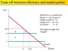
	Assuming a constant marginal cost, and p = MC under competition, illustrate how a merger could lead to the market power/efficiency trade off (by illustrating the change in CS. What is the Williamson trade-off?	So Net benefit depends on whether the square A is bigger than the triangle B. The Williamson tradeoff is the tradeoff between A and B, i.e. the producer surplus gained vs the consumer surplus lost.
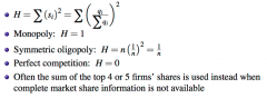
	What is the Herfindahl index? How can the index be used? What are the problems with relying the Herfindahl index?	The Herfindahl index is a measure of industry concentration. - It is the sum of squared market shares Using the Herfindahl Index: - USA: Mergers that increase H further (when H is already high) are subject to further analysis or banned ... note: this calculation assumes that the merged firm's market share will be the sum of the merging firms' Relying on the Herfindahl index to prevent mergers may not be wise since the effect of a merger depends strongly on the type of competition (often more than industry concentration) - In Cournot markets, prices and profits go up as the number of firms go down - But in Bertrand markets (with identical firms and products), p = c, and π = 0 before and after a merger, as long as at least 2 firms remain - We also care whether collusion will be made easier! - So all in all, looking at the Herfindahl index alone can be misleading...
	What are the benefits/costs of a horizontal merger?	Costs: - Consumer Surplus is lower (price rises and q falls) - Collusion is more likely with fewer firms (since δ threshold falls for collusion to be sub-game perfect), i.e. firms can be less patient to still collude - Keeping firms separate reduces future collusion possibility if firms have different cost structures; before merging, they are unlikely to collude, but together, they may be similar sizes to other firms etc. Benefits: - Cost efficiencies (what firms claim can occur), i.e. the Williamson trade-off: firm's cost savings to create profit may outweigh loss in CS surplus ... but couldn't these cost efficiencies just be made by enlarging instead of merging? ... not if the benefits of mergers are synergies rather than structural benefits from joining that could be replicated by self-enlargement - R&D: Superior profits enable money to be invested ... but this only makes sense if the firm is already capital constrained (i.e. cannot raise debt or equity) - Firms need some profit: ... encourages initial investment in the first place (e.g. like the patent argument) ... if there are zero profits, no one will invest ... if there are profits (and no barriers to entry), then firms will join - Preventing the horizontal mergers is costly, e.g. the case/lawyer fees - stop it later if you need to, but let it go ahead for now
	Explain how the effect of a merger will depend on the relevant market (market definition) using a theoretical example.	Example: - Suppose Coke and Pepsi merge - If the market is 'cola', the merged firm becomes essentially a monopolist - But if the market is simply 'bottled beverages', then the market share of the big firm is not as big, since they also compete with bottled water, bottled beer, wine, fruit juices and other soft drinks, etc.
	What are the factors considered when determining the size/definition of a market?	US Dept. of Justice 1992 Guidelines: - A market is the minimal set of products (over product and geographical space) over which a hypothetical monopolist would find it profitable to raise the price (from the non-cooperative level) The SSNIP test: - Small but Significant Non-transitory Increase in Price - This test determines whether such a prise rise would be profitable So the size of the market depends on the degree of substitutability between products. - If the cross-brie elasticity is high, then when the merged firm tries to raise its price, demand will shift to substitute products (so the merged firm alone is not a market) But the size of the market also depends on whether a price increase would induce entry of new firms, or of existing firms making related products
	What is a random experiment? What is a Sample Space What is an event? What is a random variable? What is its support? What is the expected value of a random variable? What is its variance?	A random experiment: An experiment with a variety of possible outcomes - E.g. Tossing a coin A sample space: The set of all possible outcomes of the experiment - E.g. Heads, Tails An Event: A subset of the sample space - e.g. Heads A random variable: a numerical variable whose value depends on a random experiment - The support of a random variable is the set of possible values it can take Expected value of a random variable: - The average value we would get over many repetitions of the same experiment Variance: - On average, how far away is X from its mean - i.e. the average of the (squared) distances of the random variable from its mean
	What is Jensen's Inequality?	For any concave function, the function of the expected value, is larger than its expected value of the function, i.e. E[g(X)] < g(E[X]) To help remember this: - Linear functions g have E[g(X)] = g(E[X]) - So think that, for a given linear function... - If you were to make it concave... - then the expected value of that function would be lower
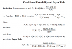
	What is Bayes Rule? Prove it.
	What does it mean for events to be independent? Why is this the case intuitively?	A and B are independent if: - P(A and B) = P(A).P(B) This implies: - P(A\|B) = P(A) - This makes sense, since if they are independent, then B occurring should not change any belief we have about A occurring
	Why is expected value an unsatisfactory criterion for choosing between lotteries? How can we get round it?	Expected value doesn't take into account risk - A high expected value may be offset in reality by a significant chance of an extremely unpleasant outcome - i.e. people seem to be bothered by the s[read of outcome and bothered more by the downside risk than the upside Instead: - we can model this effect as thinking of individuals as assessing outcomes in terms of some utility function and then evaluating the expected utility of the gamble offered (instead of raw outcomes)
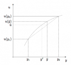
	What is the significant of a concave utility function in expected utility theory? What is the certainty equivalent? What does Jensen's Inequality tell us about it (e.g. in relation to the expected value of the outcome)	Concavity of the utility function implies: - increments to the right are valued increasingly less - This is a reflection of higher risk more offsetting a greater return - So there is decreasing marginal utility The certainty equivalent: - what the agent is willing to pay to take on a risk (that they are not already faced with)... or what the agent must be paid in order to not take on that lottery - i.e. what (certain) sum gives me the same utility that I would expect to get from taking on the lottery - u (CE(w + X)) = Eu(w + X) ➡ CE(w + X) = u⁻¹(Eu(w+x)) ...or in the insurance market (when already faced with an uncertain outcome, from which you may want to evade), it is how much the agent values the random income given up in order to receive a sure income By Jensen's inequality, if u(.) is increasing and strictly concave: - Eu(w + X) < u( E(w+X) ) ➡ but Eu(w + X) = u(CE(w + X)) so ➡ u(CE(w + X)) < u( E(w+X) ) ➡ so CE(w+X) < E(w+X) Analogously, if u(.) is increasing and strictly convex: CE(w+X) > E(w+X) If u is linear: - CE(w+X) = E(w+X)
	Define (absolute) risk averse, risk seeking and risk-neutral behaviour. What does this imply for concavity and certainty equivalents? What is relative risk aversion?	An agent is risk averse if, at any wealth level w, and for any lottery L , she prefers to receive the expected value of the lottery E(L) with sure probability instead of playing the lottery with uncertainty. An agent is risk-seeking if she prefers to play the unexpected outcome lottery L instead of receiving E(L) An agent is risk-neutral if she is indifferent between playing L and receive E(L). If Agent A is risk-averse: - uA is concave (or u'' < 0, if u is differentiable) - CE(w+X; uA) < E(w+X) Relative risk attitudes: - Agent A is more risk averse than agent B if (holding initial wealth constant across agents) for any lottery, A's certainty equivalent for lottery L is lower then B's - This makes sense, since agent A is willing to pay less than Agent B for the same risky prospect - So A's utility function will be a concave transformation of B's (i.e. it will be more concave)
	What is the risk premium?	The risk premium is the difference between the expected lottery outcome and the Certainty equivalent, i.e. RP(w + X) = E(w + X) - CE(w + X)
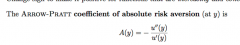
	What is the Arrow-Pratt index of absolute risk aversion?	-So if A and B have differentiable utility functions, uA and uB... - and if A's utility function is more concave than B's, then - AA(y) ≥ AB(y) - So it is a measure or ska version embodied in the utility function
	Under uncertainty, is utility cardinal or ordinal? Does this make a difference?	Utility is cardinal, since this matters for establishing the concave nature of utility functions Since these utility functions embody risk attitudes, transformations of utilities must preserve these risk attitudes - Increasing linear transformations do preserve risk attitudes don't - Others (even if they are monotonic, e.g. squaring it), does not
	Why are there gains from trade in the insurance market?	When a consumer buys insurance from an insurance company, she swaps out a random part of her income for a sure income. The Consumer: - If she is risk averse, she values this random income which she is giving up in the exchange at less than its expected value The Insurance company: - If the insurance company were less risk averse than her (e.g. almost risk neutral), then it would value the random income being offered at closer to its expected value
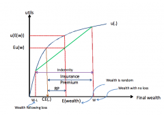
	What is the most the agent will be willing to pay as an insurance premium (if the insurance company is willing to fully indemnify the agent, if the insurance decision is a yes/no decision? Explain why.	Model: How much will the consumer pay for her premium? - Risk averse agent with random wealth: w with prob. p₁ and (w-L) with prob. p₂ (= 1 - p₁) - The most the agent is willing to pay is:w - CE, where CE is the certainty equivalent of her random wealth - If she pays this maximum amount then: ... In "good times" (no loss occurs), she ends up with w - (w-CE)) = CE ... In "bad times" (i.e. loss occurs), she ends up with w - L + L - (w - CE) = CE ... so she definitely ends up with some sure incomes which she values the same as her random income - Both the agent and the insurance company are left better off: ...She swaps her random endowment (her risk) for a sure income with the insurance company ... to the insurance company, the random endowment is worth its expected value which is greater than the CE to the agent ... So if the insurance company is (close to) risk neutral and the agent is risk averse, both agent and insurance company are left strictly better off by the swap
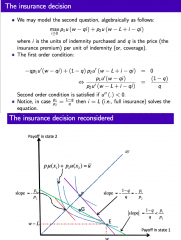
	What will be the agent's insurance premium (if the insurance company is willing to indemnify the agent), if the insurance decision is a 0-1 decision (i.e you can buy variable amounts of indemnity/coverage, at a given per-unit rate of insurance premium)?	The agent wants to maximise their expected utility: see above-maximisation problem (where p₁ and p₂ are probabilities) - Solve for FOC - (also note that SOC is satisfied if u''(.) < 0 ) Given the FOC: - if p₁/p₂ = (1 - q)/q, then i = L (full insurance) solves the equation! - but if (more generally...) p₁/p₂ > (1 - q)/q, then we need to use a state-contingent pay-off space In the state-contingent payoff space: - The two states of nature: ... state 1: the event that the loss does not occur ... state 2: the event that the loss occurs - The state continent payoff vector (w, w - L) represents the random endowment (E) Consumer: - If you buy i units (i dollars worth) of indemnity at price q per unit, you give up qi in state 1, but that is in exchange for receiving i - qi in state 2 - So the slope of the budget line that describes the agent's opportunity set (i.e. the insurance opportunity on offer) is: ... Δx₂/Δx₁ = - (i-qi)/qi = - (1-q)/q = (q-1)/q ... this is the number of state 2 dollars we can buy, per state 1 dollars The insurance company: - The rate of insurance premium q is "fair" if (on average), the insurance company just breaks even, i.e. in expected terms, on the insurance contract, ... p₁qᵢ + p₂(qi-i) = 0 ➡ q= p₂ Putting them together: - The slope of the consumer's budget line (which must go through the endowment E) is therefore now: ... -(1-q)/q = -(1-p₂)/p₂ = -p₁/p₂ - Therefore the agent's optimal choice is to purchase full insurance (POINT F) ... i.e. it is only on the certainty line that the indifference curve has slope -p₁/p₂ (this is true irrespective of the agent's risk attitudes) - If the insurance is more expensive than this fair price q, then the budget line of the consumer flattens (flatter than -p₁/p₂), the optimal purchase will then be less than full insurance (e.g. point G - should be a tangent point in diagram), since it is only below the uncertainty line, that the IC has an indifference slope flatter than -p₁/p₂
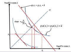
	What is a state-contingent payoff space? What is the certainty line?	State-contingent payoff space - State of the world/nature: a realisation of affairs (a resolution of uncertainty), that fixes the outcome of an action with uncertain consequences ... e.g. loss or no loss (insurance purchase example) describes two possible states ... e.g. movie A is good/bad and/or movie B is good/bad describes 4 possible (payoff-relevant) states The diagram: - A state contingent payoff space consists of points (e.g. 𝘹 = (x₁, x₂) which each describe a particulate state-contignet consumption veto - Think of state 1 and stay 2 as having probabilities p₁ and p₂ respectively ... one risk neutral agent (red preferences/IC) ... one risk-averse agent (blue preferences/IC) - the equation of an indifference curve is: p₁u(x₁) + p₂u(x₂) = u¯ (obtain slope by implicit differentiation) - the 45° line is the certainty line, i.e. getting the same outcome in each state of the world - - when the IC crosses this line, its slope is dx₁/dx₂ = -p₁/p₂ irrespective of the agent's risk attitude
	Why is expected utility reasonable? What is the independence axiom? Explain its implications, i.e. the features of the utility function that it underpins.	Expected utility formation of agent's preferences over risky alternatives is: - useful: allows us to model risk attitudes - convenient: simple, tractable model It is reasonable when the independence axiom applies, because this underpins (crucially) - separability in the evaluation of mutually exclusive outcomes, i.e. each commodity is completely separable from the evaluation of the others ... this is realistic when there is no complementarity among the commodities - linearity in probability weights used to aggregate the separate evaluations, i.e. the utility function is linear in probably weights e.g. U(x₁, x₂, x₃) = p₁u(x₁) + p₂u(x₂) + p₃u(x₃) (much simpler than a standard utility function without risk) ... this is realistic when the outcomes are mutually exclusive events The independence axiom: Separability: - One's ex ante evaluation of consumption in some contingent state should be independent of what the consumption possibility is for any other state - So the trade-off across states is independent of the consumption in any third state, as is evidence in the expected utility formula: U(x₁, x₂, x₃) = p₁u(x₁) + p₂u(x₂) + p₃u(x₃) ➡ MRS₁.₂ = p₁u'(x₁)/p₂u'(x₂) - So the MRS depends only on how you have of (contingent) goods 1 and 2, and not how much you have of good 3 - This clearly rules out complementarity (between consumption across states) - The makes sense because states are mutually exclusive events, i.e. only one or the other occurs The independence axiom: Linearity in probability weights - Consider that xn occurs with probability pn (for n: 1, 2, 3) ... i.e. (x₁, x₂, x₃; p₁, p₂, p₃) and we are shining probability to outcome 1: ... ((x₁, x₂, x₃; p₁ + Δ₁, p₂ - Δ₂, p₃ - (Δ₁ - Δ₂)) - Because the utility function is linear in probability weights, welfare is unchanged if: Δ₁u(x₁) = Δ₂u(x₂) + (Δ₁-Δ₂)u(x₃) ... this is irrespective of the starting values of the probabilities - So, how the increase in the probability of outcome 1 (Δ₁) is evaluated does not depend on the (starting) probability of outcomes 2 and 3 - This makes sense because the outcomes are mutually exclusive
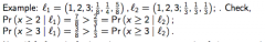
	What is the basis for comparing lotteries? What is First-Order Stochastic Dominance? (add pic)	Return: - Higher vs Lower Dispersion of returns: - Less risky vs more risky First-Order stochastic dominance: F(.) first-order stochastically dominates G(.), where F(.) and G(.) are CDFs, if: - Either: Every expected utility maximiser (for whom "more is better" prefers F(.) over G(.) - Or/and: for every amount of money x, the probability of getting at least x is higher under F(.) than under G(.) ... so 1 - F(x) ≥ 1 - G(x) at each x ➡ F(x) ≤ G(x) at each x ... so a lottery L₁ stochastically dominates L₂ if and only if there CDF corresponding to L₁ lies below the CDF corresponding to L₂ - Also, normally if L₁ f.o.s.d. L₂, then (irrespective of risk attitude) the mean outcome under L₁ is greater than the mean outcome under L₂ (but the converse is not generally true)
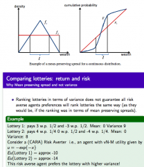
	What is a mean-preserving spread? What does this imply for variances of two lotteries? What does this look like graphically (CDF)? Why is mean preserving spread used and not variance to compare lottery riskiness?	A mean-preserving spread is a way of comparing riskiness - We can compare lotteries with the same mean (normalising them(, so that if one if chosen over the other, it s because it is less risky - A graphically, (a sufficient condition is that) the CDF of L₁ crosses the CDF of L₂ from below (and they cross just once), means that L₂ is a mean preserving spread of L₁ Intuitively: - A mean preserving spread squashes the pdf down, transferring probabilities 2 the two tails, which therefore makes it riskier - Since chances of better outcomes matter less than chances of riskier outcomes Variance Implications: - If L₂ is mean preserving spread of L₁, then the variance of L₂ will be greater than that of L₁ ... but the converse is not true - i.e. mean (L₁) = mean(L₂) and var (L₁) < var(L₂) does not imply that L₂ is a mean preserving spread of L₁ We use mean preserving spread instead of variance because: - Ranking lotteries in terms of variance does not guarantee all risk averse agents preferences will rank lotteries in the same way - Since a lottery may have a higher variance but actually "spread risk" less, take on less extreme values - so variance is not a universal measure of risk - see example above
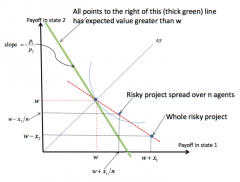
	What is the intuition behind risk-spreading? What does this look like in a graph? What is the real-world application of this?	Consider risk-averse agents with sure initial wealth w, and vN-M utility function u(.) - An agent may be offered a risky project with a positive net pay-off - But the CE may be less than initially wealth w - So the agent acting alone may not take it on But if the agent joins with other agents and each divide up the net payoffs in each state of the world: - There will be some number n such that a group of size n or larger will take on the project More generally (if net payoffs in each state are x₁ and x₂ - E(w+X) = p₁(w+x₁) + p₂(w+x₂) > w, and CE(w+X; u) < w - Then there is some n¯ s.t. for all n > n¯, CE(w + X/n; u) > w - So at some n, everyone will want to take on the project (as long as the expected payoff is positive) - As n increases, you get close to w - When n is large enough, agents can act as if they are risk neutral Real-world: - This is why we have joint-stock companies (spreading a company's risk over many people), which works so long as expected returns are positive, i.e. at points to the right of the thick green line in the graph
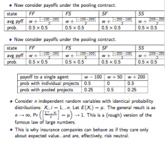
	What is the intuition behind risk-pooling?	Consider risk-averse agents with sure initial wealth w, and vN-M utility function u(.) - But each agent is offered a different risky project - Very importantly, the random variables describing the project net payoffs are independent random variables (independent risks) - So the expected net payoff for each project may be positive, but each agent may be sufficiently risk averse to not want to take on a single project - By pooling the risks, each agent draws the average project income from the pool, i.e. ∑ᵢ₌₁ⁿ (Xᵢ/n) ... where Xᵢ is the random net payoff from a single project ... where n is the number of agents/projects in the pool So as n → ∞, you are more likely to be able to actually draw the mean of the joint projects outcomes (i.e. this is unlikely/impossible with a small number of projects) - see above - this is (kind of) the LLN - this explains why insurance companies can behave as if they are almost risk-neutral
	What is the analogous nature of risk allocation to goods allocation?	The allocation of risk is analogous to the allocation or goods in a simple exchange economy - Agents may have standard convex preferences over risk (just like they can with goods), so there is a diminishing marginal rate of substituting, i.e. less income in state 1 and more income in state 2 means she is more willing to swap (ex ante) income in state 2 for income in state 1 ... i.e. agents are risk averse, and want to smooth consumption across states ... this would bring us closer to the certainty line - Swaps/exchanges can enhanced welfare because MRSs (personal rates of trade-off) differ across agents ... because of outright difference in taste, i.e. different preferences ... or because a very asymmetric initial allocation that is inefficient ... this enables ultimate consumption to be smoother than initial income/endowment - Pareto efficiency is characterised by equality of MRS's ➡ there is a market mechanism to achieve this
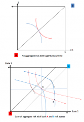
	What is the efficient allocation of risk in an exchange economy with two states?	Set-up: - Two states: s =1, 2 - Interior allocation is given by xʰ = (x₁ʰ, x₂ʰ) for h = A, B, i.e. each agent in the economy - ωᴬ + ωᴮ is the total (contingent) endowment vector in the economy Efficiency (for an interior allocation xʰ) is characterised by: MRSᴬ₁,₂ = MRSᴮ₁,₂ ➡ Note: ex-ante, so just like normal consumer theory except that we multiply by the probabilities - since the agents have the same beliefs and are both utility maximising, the probabilities are the same for each state according to each individual (so they cancel out) - the equilibrium is symmetric in terms of MRS foe each agent - i.e. u'A(x₁ᴬ)/u'A(x₂ᴬ)= u'B(x₁ᴮ)/u'B(x₂ᴮ)= Efficiency is also characterised by total consumption equalling what is available (i.e. total endowment), i.e. demand = supply, so the market clears so FTWE1 satisfied. By the FTWE, equilibrium allocation are parted optimal if the market for claims is complete. The outcome depends on the type of economy: - An economy with no aggregate risk (even though individual endowments are risky), i.e. total endowments are equal in state 1 and in state 2 - Edgeworth box is a square - Equilibrium price ratio is equal to the probability ratio (the "odds") q₁/q₂ = p₁u'h(x₁ʰ)/p₂u'h(x₁ʰ) = MRSʰ₁,₂ = p₁/p₂ - Risk is efficiently shared, since (despite risky individual endowments), the final individual consumption is rissoles (like the aggregate) - both agents certainty line coincide and this is the contract cute (in a square box) so both can be satisfied fully and neither agent bears any risk An economy that has aggregate risk, i.e. less (total) endowment in state 2 - Edgeworht bo is now a rectangle - Above A's certainty line, MRSᴬ₁,₂ > p/₁p₂ (i.e. steeper IC) - Above B's certainty line, MRSᴮ₁,₂ < p/₁p₂ (i.e. flatter IC) - So efficient allocation must lie between their certainty lines (which now do not coincide)
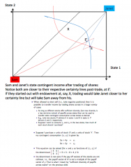
	Why does diversification make sense? What if short-selling is allowed? Are there limits to diversification?	Sam and Jane both have projects but both prefer Sam's - Sam and Janet may still exchange part of their projects since this allows Sam to diversify - This brings Sam (and Janet) closer to their certainty lines (depending on where the starting endowment is) - If the endowment is outside both certainty lines, e.g. at E, they will both be brought closer to their certainty lines (i.e. to E') - But if the endowment starts between these certainty lines, e.g. at E, then trade may not be beneficial for one investor, since they may be drawn away from their certainty lien and towards the other person's, depending on where the equilibrium outcome is (which depends on preferences of each person as it is where MRS's are equal) So: - they can both mutually benefit if their projects are diverse enough (i.e. if their initial endowment point lies outside the tram tracks created by their certainty lines (assuming no short-selling, i.e. only positive amounts of shares can be bought) - if they are outside the tram-tracks, then some swap of shares will be mutually beneficial! - this is not guaranteed if initial endowment is inside the lines - this arises because of the asymmetric payoffs of the projects ("diverse enough"), so that you can get more state 2 income and less state 1 income This is more likely if short-selling is allowed, as any allocation can now be reached by trading: - As long as the payoff vectors of the stocks are not collinear (i.e. multiples of each other), then they are sufficiently diverse - i.e. the determinant of the state-contingent consumption matrix is non-zero Limits in diversity of tradable stocks... when - there is asymmetry of information - this causes incompleteness of contingent income markets too
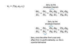
	How is the envelope theorem relevant to the Cournot Competition model with two firms?	A marginal change in a firm's own cost affects its profit through 3 channels: - the direct affect of a change in its own costs - an indirect effect via the change in its own quantity - a second indirect effect through a change in the other firm's quantity The indirect effort via the change in its own quantity will be zero, since: - ∂π/∂q₁ = 0, i.e. we know the firm is choosing quantity to maximise its own profit anyway - so (at the margin), changing the quantity by a tiny bit would make zero difference Similarly, when we examine the marginal change in the other firm's own cost, to see how it affects the first firm's profit, it again operates through 3 channels: - the indirect direct affect of a change in the other firm's costs - an indirect effect via the change in its own quantity - a third indirect effect through a change in the other firm's quantity
	Describe the market for Lemons (Akerlof) as an example of adverse selection. What does this imply for FTWE1?	There is a market for used cars, where the current owner of a car has better information about its quality than the potential buyers. - Quality of a used car, designated by some number q is distributed uniformly over [0, 1] - There is large number of demanders: each will pay 3q/2 for a car of quality q - There are a large number of sellers: each will sell a car of quality q for price q ... So if quality was observable, there would be efficient trade at some point between these reservation prices. If quality is not observable: - Buyers estimate the quality of a car offered to them by considering the expected (average, conditional on information they have) quality of cards offered in the market - So on average, buyers will be willing to pay 3q¯/2, where q¯ is expected quality Take some possible positive equilibrium price p¯ > 0 - All sellers will quality less than p¯ will want to sell their car, since p is greater than their reservation price - However, no sellers with quality greater than p¯ will want to participate in the market - So consumers now know that quality is distributed uniformly on [0, p] and not [0, 1] - So now, expected quality (conditional on the information equilibrium price p), is now q¯ = p/2 - So now a buyer will want to pay just 3q¯/2 = 3/2 x p/2 = 3p/4 - This is less than price p, the price we assumed a car would be sold at - So no cars will be sold at price p, and sellers with quality above 3p/4 will again drop out of the market (this is the adverse selection) - p was an arbitrary price... so no used cars will be sold at any positive price. Unique equilibrium is p = 0, with demand = supply = 0 The bottom line: - Any price that is attractive to the owners of goods cars is even more attractive to the owners of lemons - Selection of cars offered to the market is therefore not representative selection, but biased towards the lemons - i.e. the selection of cars is an adverse selection FTWE 1 does not work here: - GCE is where p = 0 and q = 0 - but we know efficient price is somewhere between p and 3p/2 - so equilibrium is not efficient - It is not efficient because there are not enough contingent markets for every state of the world (i.e. every possible quality) - You need something to transfer money to that state of the world
	Why does adverse selection cause credit rationing?	Credit Rationing: - There is persistent excess demand for credit - but the interest rate does not rise to clear the market - this is because this would result in adverse selection and lower the bank's net expected profits - so instead of raising the interest rate, banks ration credit - so banks limit the supply of credit even to those who are willing to pay more than the current rate A bank faces two consumers, who it cannot distinguish between: - consumer A, who will make a sure 10% return on his project - consumer B, will either make 30% or lose 10% (so there is an expected, i.e. average 10% return) ... but if consumer B loses this, and the bank has lent them money, then the bank will itself lose 10%, because there is limited liability Assume the bank can make money at 5% (i.e. the bank's reservation price is 5%) - If it gets a random selection it will lend to these consumers - If the consumer's reservation price is 10%, then an efficient equilibrium occurs at some price between 5 and 10% - Assume that a competitive equilibrium occurs at 5% (so both the bank, and consumers, on average make money), i.e. 5% is the market interest rate Now assume that conditions change int he economy such that bank would need to receive just over 10% to be profitable (if it was lending to a random selection of consumers A and B). The bank then raises the interest rate to just over 10% - Type A borrowers will no longer borrow, since it is more than their project return, i.e. they will definitely lose money (adversely selects itself out of the market) - But Type B will still borrow, since in the good state they still net 20% (30% - 10%), and in the bad state, they make/lose nothing, because of limited liability This means that if the bank raises the interest rate: - their net expected earnings fall, since they are stuck with type B consumers, who will more often than type A consumers lose them money Instead, therefore, the bank may prefer to retain credit: - this involves, e.g. asking for collateral
	Why can information be valuable?	I have two career path choices: - teaching, which is safe, and guarantees me an income of 5, and an associated utility - acting, which is risky (reward of 400 if i become a star, or a reward of 2) - Absent information, I would choose to become a teacher, if my utility of income from teaching is greater than the expected utility of income from acting However: - If i had more information (e.g. about whether I could become a star), then this may affect the actions I take - I would therefore be willing to pay up to a certain amount for that information - If I were to pay for information though, this could not lower my expected utility below my safe bet if I dont seek information and just become a teacher - Therefore at the limit, I would be willing to pay for information, such that my expected utility from seeking information (and then becoming an actor, or then becoming a teacher with this information in hand) is equal to my utility if i dint receive this information at all, and just became a teacher The role of information: the bottom line - Information that helps to reduce uncertainty has economic value - It has such value because it allows the decision maker to adapt her action to the true state of the world, i.e. to choose an action that is more appropriate to the true state of the world - The value of information is entirely instrumental: it arises only because it allows us to choose a better action (i.e. we use it as a means of achieving something else) ... i.e. the one that gives us a higher payoff int he true state of the world
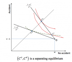
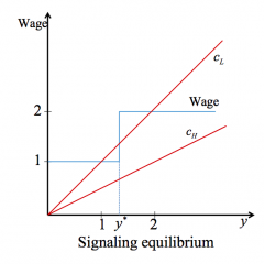
	How can adverse selection situations be overcome by the use of market signals? What is a separating equilibrium? - Why is it a Nash Equilibrium? What is a pooling equilibrium? Discuss the welfare properties in each equilibria (i.e. for each agent, and the firm) Crucially, why is a signalling equilibrium possible?	- The signal takes the form of an action that has economic consequences - Observation of the action an agent takes may then reveal his private information (I.e. his "type") that is otherwise hidden Separating equilibrium: - An equilibrium where each "type" takes a different action (i.e. a different amount of the signal) - This then reveals their private information (their "type) Job Market: - Pay wage of 1 to employees with education level below y* - Pay wage of 2 to those with an education level above y* and above (remember that the marginal cost of acquiring y units of education differs for each type) (fraction q are of type low productivity, paid 1 in full information, and factor 1-q are of type high productivity, paid 2 in full information) ... the average marginal product is 2- q, so this is what the "average" pay/marginal product would be in competitive markets with full information - Given this wage schedule, individuals select the level of education that maximises their net return (i.e. wages minus cost of education) - literally just look for the biggest gap between the wage schedule and the cost of education schedule Nash Equilibrium: - Individuals have no unilateral incentive not to take these separate signals - firms satisfy the zero profit condition, since they are paying the marginal product to each employee - but this separating nash equilibrium is not unique, since (in our example) and y* between 1 and 2 yields a separating equilibrium ... y* = 1 is the most efficient, since it still enables each type to self-select, but maximises the net profit of both consumer, especially the high productivity worker, who now enjoys greater profit Pooling equilibrium: - where all types of agents take the same action (here, you wouldn't be able to tell who's who) - e.g. a flat pay rate of 2 - q, i.e. the average expected marginal product/wage (irrespective of the level of education undertaken) would cause both agents to choose y = 0 (makes sense: why would i bother to spend on intrinsically useless education if it doesn't get me more money?) - this means the firm has just as much information has it had to start with (none!) - i.e. same as equilibrium without signalling - here the information/signal has no instrumental value, since it doesn't differentiate you Welfare Properties: - Low productivity agents are worse off in the separating equilibrium (compared to the pooling equilibria) since their wage is reduced from (2-q) to 1 - Within the set of separating equilibria (i.e. q* at some level between 1 and 2), high productivity agents are made worse off as y* is increased, since their wage remains the same, but their signalling costs increase. Depending on how low q is (which affects their wage in the pooling equilibrium), they may even be worse off than they were in the pooling equilibrium... so both could be worse off in the separating equilibrium - Firms make zero profits in all equilibria, since they pay agents the revenue of their marginal product Signalling equilibrium is possible because: - the marginal cost of taking the signal action is different for each "type" - This makes the signal credible - In a separating equilibrium, H types must pay for the cost of the signal they undertake, which has no intrinsic benefits - Welfare effects are ambiguous if information has no instrumental value
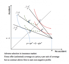
	In an insurance market with asymmetric information, why does adverse selection occur when contracts only specify a rate of premium?	Assume: - there are good-risk types and bad-risk types of consumers with probability of accident πᴳ & πᴮ - the average probability of accident is p¯ = qπᴳ + (1-q)πᴮ - Types are private information - Sellers are risk neutral - Buyers are risk averse expected utility maximisers with identical vN-M utility - At any arbitrary point, the slope of type G's indifference curve is steeper than type B's, since when you differentiate to get the MRS it depends on (1-π)/π ... intuitively, good-risk types care less about state 2 income, since their state 2 (having an accident) is less likely to occur When only the rate of premium is specified, adverse selection occurs because: 1. Price offered is between πᴮ and p¯ ... because the average probability of accident is p¯ in the population, then the seller needs to charge at least p¯ to not make a loss ... but any price up to πᴮ would be greater than the likelihood of the good types having an accident ... therefore the good types will only partially insure themselves (partially adversely selecting themselves out of the market) ... the bad types will fully insure themselves, since they are paying below the fair price of their probability of accident ... the firm therefore has negative expected profits, since there are not enough good risk types to not take put enough insurance to balance out the bad risk types ... so there is no equilibrium with non-negative expected profits 2. The price offered is πᴮ. ... now only bad risk types will buy insurance, and good risk types will fully select themselves out of the market. ... this is the classic lemons outcome ... this is an equilibrium with zero profits - only bad types are involved, and they are fully insured at their reservation price
	What is screening, and how is it different to signalling?	Signalling: - Individuals on the more informed side of the market choose an action to signal information about their abilities to uninformed parties Screening: - The uninformed parties take steps to try to distinguish (screen) the various types of individuals on the other side of the market - e.g. Rothschild and Stiglitz (1976) in insurance markets: 'at this price, you can have "this much" coverage'
	In an insurance market with asymmetric information, if firms offer price/coverage packages, what will this look like graphically?	Graphically: - insurance companies will offer only points in the contract space (rather than a line, which occurs when just a price was a given and the consumer chooses her desired coverage) - An insurance contract consists of a pair (ɑ₁, ɑ₂) where ɑ₁ is the total premium paid, and ɑ₂ is the net compensation paid in case of an accident ... so for z coverage, the equivalent price is: ɑ₁/(ɑ₁+ɑ₂) ... this gives a slope of the "budget line" of - ɑ₂/ɑ₁
	What is a Rothschild-Stiglitz Equilibrium? - is this a Nash equilibrium? What are the different types of possible contracts?	A Rothschild-Stiglitz equilibrium is an equilibrium in a competitive market where firms offer price/coverage packages. - A set of contracts is an equilibrium set of contract if: 1. all contract pairs (of price and coverage level) are offered earn an expected profit of 0 2. there is no other contract that could be added to the equilibrium set of contracts that would earn a positive expected profit ... this is a Nash equilibrium among insurers (where each insurer's strategy is a set of insurance contracts offered) There can be two types of contract: - pooling contracts, (ɑ₁, ɑ₂) intended for all agent types - (a menu of) separating contracts { (ɑ₁ᴮ, ɑ₂ᴮ) , (ɑ₁ᴳ, ɑ₂ᴳ) } which lead to self-selection But there does not exist an equilibrium with pooling contracts: - Since there is zero expected profit, pooling contracts on offer must be on the actuarially fair price line, i.e. corresponding to the price p¯ = qπᴳ + (1-q)πᴮ, e.g. at point C - At this price in between πᴳ and πᴮ, good risk type agents only partially ensure themselves - So there is an incentive for one firm to deviate and offer a lower price, closer to πᴳ, e.g. a line that would go through C'. ... this is now off of the actuarially fair price line, and so would entail positive profits ... therefore no such pooling equilibrium could exist as a Rothschild-Stieglitz equilibrium since another positive profit equilibrium would be possible What about a separating equilibrium: - There is menu of two contracts, such that buyers self-select themselves into choosing the contract intended for their type ... { Cᴮ = (ɑ₁,ᴮ ɑ₂ᴮ), Cᴳ = (ɑ₁ᴳ, ɑ₂ᴳ) } - It must be in the self-interest of each type to select the contract intended for the type and not that intended for the other type ... so contract B must be preferred to contract G by consumer type B .. but contract G must be preferred to contract B by consumer type G - Cᴳ must lie on the price line corresponding to πᴳ, and Cᴮ must lie on the price line corresponding to πᴮ - this ensures that the firm makes zero profits - Cᴮ must lie on the 45° line, since otherwise they could be better off (type B utility is maximised on the certainty line, since they are so much worse off in state 2... whereas type G would prefer to hedge their bets and be closer to the BR of the graph) - So Cᴮ is determined (45° line and on the appropriate price line). Now we just determine Cᴳ by ensuring that it is on its appropriate price line.
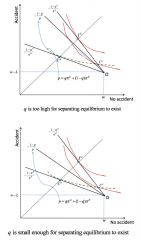
	Will a separating equilibrium in the insurance market with asymmetric information always exist?	No - this depends on the average probability of accident in the population. - If q (the proportion of good-type agents) is high, then the average probability of accident will be lower, so there average price will be lower. - This causes a steeper price line. If it is so step so as to intersect the indifference curve of type G passing though Cᴳ, then... ... any contract in the shaded area will then be accepted by both types of agents and gives strictly positive profits to companies offering it If q was lower: the line corresponding to this price will lies everywhere below the IC of type G passing through Cᴳ. Then existence of a separating equilibrium is assured. So when a separating equilibrium exists: - bad risk types are fully insured - good risk types get partial insurance The bottom line: - the fact that it is relatively cheaper for G types to decrease coverage is used to screen types. - this i just like in the signalling case where the difference in MC of acquiring a signal was used to create a separating equilibrium
	There is a two-state Principal-agent problem: - agent is risk averse with utility u(w, e) = u(w) - e, u' > 0, u'' < 0 ... the agent's income is his wages w ... the agent can choose effort eᴴ or eᴸ, which is private information - the principal is risk neutral ... P's profit is the net income of the firm (i.e. gross profit minus wages paid to A, i.e. x - w) The state of the world determines the firm's gross profit - but the probability of a state occurring is determined by A's effort - state i, occurs with probability πᵢᴴ or πᵢᴸ depending on effort level - P offers A a wage contract specifying wages in each state of the world. If the agent does not accept this contract, he gets some level of reservation utility, u¯ What is P's maximisation problem? Assuming that the constraints bind, what is the implication of agency costs for each party? How does P incentivise A to take on the high effort level?	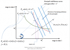States: n = 2 Profit in each state: x₁ > x₂ Probabilities: 0 < π₁ᴸ < π₁ᴴ < 1 Assuming that P wishes agent A to implement effort eᴴ: max w₁, w₂ [ (x₁ - w₁)π₁ᴴ + (x₂ - w₂)π₂ᴴ ] s.t. - Participation Constraint (PC) ... u(w₁)π₁ᴴ + u(w₂)π₂ᴴ - eᴴ ≥ u¯ ... this states the agent's ex ante expected (net) utility from participation exceeds his reservation utility that he would receive from non-participation ... so this ensures that the agent takes the contract - Incentive Constraint (IC) ... u(w₁)π₁ᴴ + u(w₂)π₂ᴴ - eᴴ ≥ u(w₁)π₁ᴸ + u(w₂)π₂ᴸ - eᴸ ... this states the the utility from taking eᴴ exceeds the utility from taking eᴸ ... this actually ensures that the agent has the incentive to take effort eᴴ Note: in Diagram, "expected" incomes are on 45° line Agency costs: - A's possession of information about his choice of effort makes A no betteroff (gets expected income at R in either case) and P strictly worse off, since P is forced to get expected income at L instead of R(compared to the case P can observeeffort). - Thus there is an agency cost, or cost of asymmetricinformation to the less well informed party P which confers no benefiton the better informed party A. - It is a loss in efficiency, a leakage ofsurplus from the relationship, unrealized gains from trade. - The agency cost is the difference in P's expected income from heroptimal contract under symmetric information with that underasymmetric information. Incentives: - In order to incentivise A to take the effort he finds costlier, P mustexpose A to risk (by making his wages vary with output). - But Adislikes risk, and needs risk premium as compensation. - This is the extracost of implementing effort under moral hazard: the agency cost.
	What is General Competitive Equilibrium?	- General:description of entire economy… many households, producers, and goods - Competitive:all economic agents are price takers - Equilibrium:Find prices such that all economic agents (households, firms) make privatelyoptimal decisions and these decisions are consistent (S=D) - 1good, S=D in 1 market à partialequilibrium - Ngoods, S=D in N markets à generalequilibrium - Assume1 county, 1 time period, no uncertainty and no government - Alsoreferred to as Walrasian Equilibrium All agents do their own things (rationally optimising objectivefunctions given exogenous prices), and these are all somehow mutuallyconsistent so that Supply = Demand ineach market; this is done by pricesadjusting. ONE MAJOR CONDITION: Thereare markets for everything (completeness à no externalities à efficient)]so… o Householdschoose consumption to maximise utility (solve à sub. budget constraint into utilityfunction... and à setwage = MPL) o Firmschoose production to maximise profit (solve --> sub. production function into profitfunction… and --> set MRS = price ratio)(Varying pricesfor above two points… will trace out supply and demand curves o Profitsare distributed to households according to some rule o Supplyequals demand for each good (i.e. each input and output) o Pricescontrol everything (they make the individual plans of households and firmsconsistent) Equilbirum is a set of prices and quantities such that supply=demand.
	What is Walras' Law? What is the Contract Curve?	Walras’ law:Value of excess demands sums to zero… o Impliesthat if there is equilibrium in (n – 1) markets, there must be equilibrium innth market too o Setone price as the numeraire since only relative prices matter Contract Curve: o the locus ofpoints where MRSa = MRSbEquilibriumlies on the contract curve (exactly where, depends on endowments and preferences)
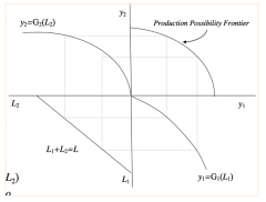
	What is the Specific Factors model? How would you use it to find the Autarky Equilibrium?	- 2 producingsectors, 1 consumer - Fixed endowmentof labour which can be used for production of good 1 or good 2 - Factor marketwill clear, such that all labour is utilised - When put intoproduction functions, these together give the PPF once you vary the division oflabour - Thismechanically derives the PPF (when you start in the BOTTOM-LEFT QUADRANT) - Assume eachproduction function is concave, since there is diminishing MPL because the otherfactor (i.e. capital) is sector specific --> only labour is sector-mobile Then treating PPF as supply… overlay the economy demand, and then find the autarky equilibrium
	How would you graphically represent a 2-person, 2-good exchange economy? How would you find each consumer's demand function? What is the Contract Curve? Where is Equilibrium? - does it always exist? - what is the core? How does the number of players affect the outcome?	Graphically: Use ofEdgeworth box, where length and width are equal to total endowments of good 1and 2, with each consumers’ endowment measured individually form theirrespective opposite corner Consumers bothchose consumer of each good to maximise utility subject to their budgetconstraint --> Using FOC (MRSa = priceratio and MRSb = price ratio) and the budget constraint gives demand function) The contract curve is the locus of points where MRSa = MRSb Equilibrium lies on the contract curve (exactly where, depends on endowments and preferences) Equilbirum is price ratio such that supply=demand(consumption of good 1 = endowment of good 1... and using Walras’ law, the samegoes for good 2). - Assumingcontinuity and strict convexity, a unique equilibrium always exists - The core is the set of all allocations which are not blocked by any possiblecoalition ... (where blocked allocations are thoseallocations which, if offered, would be rejected by a coalition because theycan gain a Pareto improvement by trading amongst themselves (or, in the case ofa single-player coalition, by retaining what they have) ... all points outside the initialIC lens (defined by their endowments?) are blocked by the single playercoalitions, and anywhere within this lens not on the contract curve can beimproved upon by the coalition of two players trading. Therefore, the coreis the equilibrium as defined above Does the number of players affect the outcome? - Regardlessof the number ofconsumers, the competitive market equilibrium is always in the core - Asthe number of consumers increases, the set of allocations in the core shrinksuntil, in the limit, it contains only the competitive market equilibriumallocation(s)
	Assume: - you can trade internationally at world prices p₁ʷ and p₂ʷ - there is one time period If you produce y₁ and y₂ and consume c₁ and c₂. - what is the economy's budget constraint that dictates their consumption? What does it mean to have comparative advantage in a good? What does this imply for its "Pattern of trade"? Is there gains from trade when the above pattern of trade holds?	p₁ʷ(y₁ – c₁)+ p₂ʷ(y₂ – c₂) = 0 1. A country has a comparative advantage in good 1 if it is relatively cheaper underautarky than free trade, i.e. p₁/p₂ < p₁ʷ/p₂ʷ (only relative prices matter). 2. Patternof trade: Each country exports the goods in which it has a comparativeadvantage 3. Gains from trade: Trade enlarges theconsumption possibility set and enables the consumers to get on a higherindifference curve
	What do the 1st and 2nd fundamental theorems of welfare economics formulate?	1stand 2nd Fundamental Theorems of Welfare Economics rigorouslyformulate the idea that, when agents act alone according to their own gain ledby an invisible hand, this actually leads to some sort of ‘good’ outcome – individual decisions can lead to ‘good’outcomes
	Social Preferences: What are social states and social orderings? Under what conditions is a social welfare ordering a social welfare function? What properties could the social welfare function have?	- Socialstates, x (complete description of the entire economy… everythingyou can imagine about it) -Socialwelfare ordering, is what orders these social states. If it is complete,transitive and continuous, then it is a socialwelfare function, SWFs could have the following properties: - Individualism/Paternalism:Defined over individual’s preferences over social states - Benevolence:increasing in each individual’s utility (not "malevolently" decreasing) - Utilitarianism:based on aggregation of total utility (requires utility is cardinal/comparable) - Rawlsian:based on utility of poorest person (as above)
	What is the Pareto Criterion? What is Pareto Efficiency? What is a utility possibility set? - where are the pareto efficient points in the set? Is Pareto efficiency a "complete" ordering? Why? What is true of MRSs and MRTs at the efficient allocation? - what does this mean intuitively?	ParetoCriterion: A social outcome x’ is Paretosuperior to x if no one finds x’ worse than x and at least one person findsit strictly better. Pareto Efficiency: A social outcome is Pareto efficient if there is no otheroutcome Pareto superior to it. Utility possibility set (drawn above) is the set of feasible utility levels that society can achieve. - Pareto efficientpoints are those on the frontier Pareto efficiency is a incomplete ordering: - any 2 Pareto efficient points arePareto incomparable. - Also, it says noting about inequality. At a Paretoefficient allocation, for any pair of goods, i, j, any pair of households, a,b, and any firms producing/using the goods MRSªᵢj = MRSᵇᵢj= MRTᵢj (i.e. opportunity costs lined up amongst agents)
	What are the fundamental theorems of welfare economics? How have they been mis-used/mis-stated for ideological reasons?	First Theorem of Welfare Economics: General Competitive Equilibrium isPareto Efficient - AtEquilibrium, consumers choose quantities such that MRSʰij= pi/pj for all h, and firms choose quantities such thatMRTij = pi/pj in production. - Sinceall agents face the same prices, the condition or Pareto efficiency aresatisfied (i.e. MRT = MRSs) ... However,note that General equilibrium would not generally be efficient if agents faceddifferent prices, e.g. with taxation (wedge between prices) or monopoly power(also a difference in prices) - so GCElies on the contract curve (CC is where MRSs are equal --> GCE is Pareto efficient) ... selfish non-communicating people leads to Pareto efficiency Second Theorem of Welfare Economics: - If preferences and production sets areconvex, then any particular Pareto efficient allocation can be achieved as a GCE withappropriate initial endowments (i.e. if you start in the right place, you can reach a particular pareto efficient allocation) - To do this,shift endowment using a lump-sum tax/transfer before trade happens (to avoiddistorting anything) - Thensociety will trade until they reach a Pareto efficient point (on the contract curve) - This theoremrequires convexity in order to reach Pareto efficiency via the price mechanism(otherwise, utility maximising and profit maximising points do not coincide --> firm will produce nothing) Mis-stated: FTWE1: “Marketsalways gets things right”FTWE2: “Canseparate equity from efficiency” ... in actual fact, theorems only hold if along list of conditions are satisfied, i.e. perfect competition, no externalities,no increasing returns to scale, no public goods, no distortionary taxes, fullset of markets, flexible market-clearing prices - also Pareto efficiency says NOTHINGabout income distribution
	What is a Social Choice Rule? What is Arrow's Impossibility Theorem? - How does majority voting fit into it? - Can we relax any of the properties in this theorem? Explain the median voter theorem in majority voting? - what is the principle of minimum differentiation?	Whenindividuals have preferences over social states (complete descriptions ofallocations) - a Social Choice Rule isa way of aggregating household utilities into social preferences Arrow’s Impossibility Theorem: No complete transitive SCR exists whichsatisfied UPID (which are potentially desirable properties of an SCR - Unrestricted Domain: works for all possibleindividual preferences - Pareto Principle: If x is preferred to x’ by atleast one individual and no individual prefers x’ to x, then x is sociallypreferred to x’ - Independence of irrelevant alternatives: In choicebetween x and x’, consumer preferences over x’’ are irrelevant - Non-Dictatorship:‘Dictatorship’ if one individual is always decisive …e.g. MajorityVoting satisfied UPID, but it is not transitive Can we relaxany properties? - Relaxing U, makes majorityvoting produce a social ordering if preferences are restricted to be‘single-peaked’ Median VoterTheorem: If alternatives are one-dimensional (i.e. along a spectrum?) and allvoters have single peaked preferences, the outcome of majority voting is thepreferred option of the median voter (the median voter is almost like adictator… whoever the median voter is, will win!) - The Principle of Minimum differentiation: If there are two parties, they will both end up offering the same platform (thatpreferred by the median voter) ... so that this becomes defined as the median voterand they are guaranteed to win… occupying the centre ground
	What does quasilinear utility imply?	Assume utility is liner in good 0, but normal (convex?) everywhere else: - there is only an income effect over good 0 - there is no income effect over any other good
	What does elasticity of supply/demand imply for policy?	DWL increases inelasticity, so just impose distortions where elasticity is lower (e.g. land),where εs = 0. - Intuition: no DWL, since behaviour doesnt change (changes in quantities supplied/consumed is small)
	What does it mean for a good to be non-rival or non-excludable? How would you see whether the markets allocate these goods efficiently? - For a good that is rival and excludable, does the market allocate efficiently?	Non-rival: zero opportunity costof consuming - "If i eat it, you can still eat it too" Non-excludable: unable to stoppeople from consuming (or producing, catching, etc) - "the supplier cannot prevent you from just taking it" To see if the markets allocate these goods efficiently: - find the equilibrium allocation (i.e. normal maximisation) - and compare it tothe efficient allocation (where marginal costs/benefits equalise?) Rival and Excludable: - Equilibrium: u’(x) = C’(x) - Efficient:u’(x) = C’(x) …. (from W = u(x) – C(x) )…. Here, equilibrium is efficient, since this maximises producer and consumersurplus
	What is the definition of a public good? - what is a pure public good? - Give an example of a pure public good? What is the equilibrium in the market for a pure public good? - What is the efficient outcome? What is the Samuelson Rule?	Apublic good has zero opportunity cost of consumption (non-rival) - Some are non-excludable (‘pure public good’) - Some are excludable - NB: not the same as a publicly provided good An example of a pure public good: defence Equilibrium: - The firm providing the public good cannot earn any revenue - so there is zero supplied by the market Efficient: - Many consumers, who all consume same amount, c1 = c2 = ….= x - If W = ∑h [ uh(x)– C(x) ], then ∑h ∂uh(x)/∂x = C’(x) The Samuelson Rule is just the rule to reach efficiency described above: - Provide x to level at which sum of marginal benefits =marginal cost
	Consider a public good that (non-rival) that is excludable - give an example. More generally, when considering efficient and equilibrium outcomes of public goods - what are the two questions we must consider? What happens under equilibrium and efficient outcomes with a public good? What is the implication for the provision of public goods by the private sector?	Example: toll road, or a park with an entry fee Questions to consider: 1. Are people excluded? 2. How much should we supply? Efficient: - Provide free access, as there is a zero opportunity cost --> people are not excluded - Provide an amount according to the Samuelson rule: ∑h ∂uh(x)/∂x = C’(x) Equilibrium: - to profit maximise, the supplier will charge a positive price, so some people will be excluded --> this is inefficient - Their revenue will be less than the full social benefit (I don't understand this part!), so there is a tendency to undersupply Implication: Public goods are not supplied efficiently by the private sector
	How could the inefficiency of the provision of public goods be mitigated? What are the issues with this?	Inefficiency mitigated if the supplier can price discriminate Perfect Price discrimination: - Personalised price set equal to h’s willingness to pay - Price to consumer his ph = u(x) + αh - ε (i.e. just below their actualvaluation) - no one with positive benefit excluded - u’(x) = C’(x) --> Producer capturesentire benefit à makes socially efficient choice Distributional issues (consumer surplustransferred to producer) Also in practice, how can you get the info for price discrimination - unrealistic as youdon't know the price but… perhaps discounts for advance booking --> late-comers have highWTP
	What is an externality? When the equilibrium outcome is inefficient because of an externality, what policy responses are there? What is the Coase Theorem?	Anexternality occurs when one economic agent’s actions affects another directly,rather than through a market - It is generally a by-product of an action that brings privatebenefit Policy responses: 1. Taxation: Set tax t* = L’(x) ….. where L(x) was the loss to the consumer Pigovian* tax, designed to counter an externality 2. Quota (or number of licenses): direct quantity control, x* a. Achieves efficient quantity b. Many firms – micro-management? These methods (Pigovian Tax and Quotas) are: - Equivalent when they use the same priceand quantity, t* and x* (in both cases too, the government gets the ‘rent’,through taxes, or auction of quotas) - But not equivalent if there isimperfect information (if policymaker does not know exact loss/cost function,then will not achieve the efficient outcome) 3. Internalise: Affected parties collectively buy thepolluter and ensure it takes L(x) into account in its optimisation 4. Bargaining: a. Affected parties collectively bribe the polluter toproduce less. Willing to pay up to L’(x) for the marginal unit, so efficient b. Firm pays households to allow it to pollute. Householdsrequire payment of L’(x) for the marginal unit Case Theorem - Under the "Bargaining" policy response, (a) and (b) are equivalent exceptfor income distribution. - Whethereach cold occur depends on propertyrights ... i.e. does the firm have the right to pollute, or the householdsthe right to clean air? ... i.e. FTWE2: Bargaining achieves Pareto efficientallocation, but which one depends on endowment of Property rights
	How does Cost-Benefit Analysis come into a government's decision to undertake a project? How will commercial decisions evaluate a project relative to the government?	Government should undertakeproject if present value of net benefits are positive - Discounted using a Social Discount Rate:society’s value of future relative to present ... higher discount rate means that we care less about future generations Commercial decisions willunderstate benefit - since they will not include the other social benefits in theircalculations

Share This Flashcard Set

Set the Language

Related Flashcards

Microeconomics

Add to Folders

Upgrade to Cram Premium

Card Range To Study

96 Cards in this Set