![]()
![]()
![]()
Use LEFT and RIGHT arrow keys to navigate between flashcards;
Use UP and DOWN arrow keys to flip the card;
H to show hint;
A reads text to speech;
29 Cards in this Set
- Front
- Back
|
Key Ideas |
The Consumption Function Marginal Propensity to Consume (MPC) Types of Expenditures Autonomous Expenditures Aggregate Expenditure Line Aggregate Demand Curve Simple Spending Multiplier |
|
|
Aggregate Expenditure |
measure of sum of all the expenditures by an economy - measure of GDP as a function of income Y = C + G + I +(X - IM) Y = GDP C = Consumption G = Govt. Spending I = Investments X = exports IM = imports (X - IM) = net imports |
|
|
The Consumption Function |
The consumption as a function of disposable income if disposable income increases, so will the consumption DI = Savings + Consumption Y - NT = DI |
|
|
Marginal Propensity to Consume |
Slope of the Consumption Function - the % of the disposable income that people are spending on buying stuff (not saving) MPC = Δconsumption / Δincome |
|
|
Non-Income Determinants of Consumption |
- things other than income can also affect consumption - these will shift the consumption function up/down i) Net Wealth ii) Price Level iii) Interest Rate iv) Expectations |
|
|
Autonomous Variable |
the variable that is not affected by a change in income |
|
|
Net Wealth & Consumption |
- stock variable - increase in net wealth will shift the CF upwards |
|
|
Price Level & Consumption |
- when price level increases so does the real value of money - if price level goes up, the $20k in your bank can buy less - people able to buy less therefore consume less Price Level ^ = Consumption Function \/ Price Level \/ = Consumption Function ^ |
|
|
Interest Rate & Consumption |
- higher interest rate results in houses saving more and spending less - CF goes down - lower interest rate results in households spending more - CF goes up |
|
|
The Life Cycle Hypothesis |
i) Young people borrow money for education & housing ii) in middle age people pay of debt & save more iii) in old age people draw down savings - net savings over life time stays the same - hence fraction of saving in an economy stays the same |
|
|
Investments |
spending on i) factories, office buildings, equipment ii) new housing iii) net increase in inventory |
|
|
Govt. Spending |
spending on g/s by the government(not including transfer payments) |
|
|
Interest Rate for Expenditure |
opportunity cost of firms investing in capital |
|
|
Investment Demand Curve |
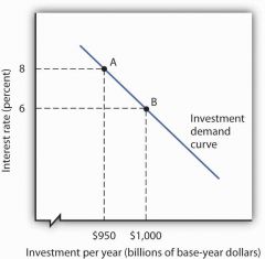
- people more interested in investing if the opportunity cost is lower lower interest rate - more demand for investments |
|
|
Investment Function |
- investments depend on interest rate and not disposable income - it is autonomous - certain factors can shift the line up and down - constant in aggregate expenditure formula |
|
|
Non-Income Determinants of Investments |
Market Interest Rates - if interest rate goes up, investments goes down Business Expectations - if business expects more profits, they will invest more (IF goes up) |
|
|
Govt. Purchase Function |

Autonomous - not affected by income (constant in the aggregate expenditure formula) |
|
|
Net Exports |

Autonomous - when Canadians have more money we buy more from other countries - when other countries have more money they buy more from us |
|
|
Aggregate Expenditure |
Expenditure method of calculating GDP Components: Consumption (C) Govt. Spending (G) Investments (I) Net Exports (NT) C increases with income (linear) G, I, NT are autonomous and constants in the equation Aggregate Expenditure = C + I + G + NT C = 𝘾 +b(Y - NT) |
|
|
Aggregate Expenditure Line (AEL) |
Equation: [𝘾 + b(Y - NT)] + G + I + NT shows how much all aspects of economy spend - since C is the only changing variable, slope of AEL is slope of C which is MPC Equilibrium point is AE = GDP |
|
|
Spending Exceeds GDP (AEL) |
- spending exceeds GDP - consumption exceeds production - more demand than supply - usually price would increase ,but in AEL price can't increase - production increases to accommodate the greater demand |
|
|
Spending is Less than GDP (AEL) |
- GDP exceeds spending - consumption is less than demand - more supply than demand - usually price would drop but in AEL price can't change - firms cut down on production instead |
|
|
Simple Spending Multiplier |
Assume Same Price Level If the spending increases, the GDP will increase by a certain multiple of the spending increase. This is dependent on the MPC. 1 /1 - MPC Example: MPC = 0.8 Spending Increase by $20B 1/1-0.8 = 5 GDP increase by 5(20) = $100B |
|
|
Spending Increase Cycle/Rounds |
1. Spending somehow increases 2. Firms produce more to match the GDP with the Expenditure increase 3. Firms producing more causes incomes to rise which causes Expenditure to rise 4. Repeat |
|
|
Aggregate Demand Curve (ADC) |
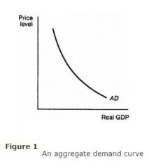
Expenditure is the demand via consumption. We calculate the different expenditure at different price levels and plot them on a Aggregate demand curve. |
|
|
Higher Price Level on ADC |
a higher price level - money is worth more and buys less - buy less = less consumption = lower expenditure - expenditure line shifts down so GDP goes down |
|
|
Lower Price Level on ADC |
lower price level - money is worth less and buys more - buy more = more consumption = higher expenditure - higher expenditure means GDP goes up |
|
|
Aggregate Expenditure v/s Aggregate Demand |
Aggregate expenditure shows the different spendings of economy at a fixed price level Aggregate demand show shows the GDP at different price levels |
|
|
Shifts of the Aggregate Demand Curve |
If the aggregate expenditure curve at one price level changes (due to consumption increase or other constants) , the aggregate demand curve will also shift for the whole economy. |