![]()
![]()
![]()
Use LEFT and RIGHT arrow keys to navigate between flashcards;
Use UP and DOWN arrow keys to flip the card;
H to show hint;
A reads text to speech;
217 Cards in this Set
- Front
- Back
|
Unemployment rate measure |
-aggregate market labor activity and -degree that labor force is utilized |
|
|
Employment and labor force participation rate |
fraction of working population that are employed and in labor force |
|
|
Unemployment rate |
fraction of labor force -searching for a job -out of work -U/LF -includes temp. layoff and waiting to start new job |
|
|
labor force |
- 15 years and older - participate in labor market activities - E+U |
|
|
Labor force participation rate (LFPR) |
-LF/POP -fraction of eligible population that participates in labor force |
|
|
Employment rate |
E/LF |
|
|
Labor Force Survey(LFS) |
-monthly - |
|
|
Employment Insurance Claimants |
-estimate how many unemployed |
|
|
EI>LFS |
Some people collecting EI but not actively looking for work |
|
|
EI < LFS |
New job seekers EI has ended |
|
|
Measuring unemployment |
-hard to distinguish unemployed vs. not in labor force |
|
|
Marginal labor force attachment |
wish to work but not classified as unemployed |
|
|
phenomenon of discouraged workers |
recession |
|
|
claim to be unemployed |
to receive financial assistance |
|
|
Issues in Unemployment rate |
-claim to be unemployed for EI while not looking -layoff longer than 6 months -Involuntary part time workers |
|
|
Stock flow model |
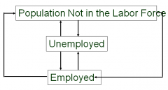
-stock for each -simultaneous flow in and out -rate of flow impact E |
|
|
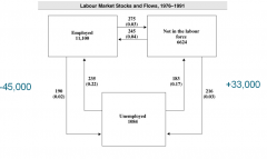
Flow |
occur each month between labor force of E, U, and not in labor force - 235000 U -> E - 190000 E -> U -ave net monthly flow 45000 |
|
|
Labor force dynamics |
|
|
|
Incidence of unemployment |
Proportion of who become unemployed in any period -probabilty of becoming unemployed |
|
|
Duration of unemployment |
length of time spent in unemployed until obtaining employment or leaving labor force -time expected to remain unemployed |
|
|
Amount of unemployed |
UR= D*I |
|
|
Unemployment in Canada |
-duration short -observed at anytime -is long term -most U is small group of workers unemployed for long D -highest U age group: longest D -very young: high prob of U -older: low U: high D -women and men similar U -avg D : 4 months |
|
|
Unemployment policy |
U caused by employment instability not shortage of jobs -most people can find acceptable job quickly -employment spells followed by job search or exit LF -still most U is the small group with longest D : concentrated |
|
|
Discrimination reasons |
- preferences - Erroneous information - Statistical judgement |
|
|
Who discriminates |
-Employers - male coworkers -Customers - unions |
|
|
Demand theories of discrimination |
demand for female labor is lower than male labor -low employment and wage -prejudice and underestimation |
|
|
Employ women if |
Wm/Wf = 1 + d d: discrimination coefficient. cost in hiring women |
|
|
Supply theories of discrimination |
Increased female supply of labor -lower productivity and low wages -Crowding hypothesis |
|
|
Crowding Hypothesis |
Females segregated to female type jobs -excess supply of female labor -lower marginal productivity and low wage |
|
|
Queing theory |
Firms pay higher than competitive wage to reduce turnover, improve moral, have queue of workers waiting to be hired at any time -women seen has higher turnover |
|
|
Statistical discrimination |
Use statistics about average to predict an individual -also used in insrurance |
|
|
Employers use a test to hire |
test may be biased |
|
|
Vicious cycle |
-Employers think women are more likely to take time off -women not promoted -opportunity cost for men becomes larger -women take time out for household -statistical discrimination |
|
|
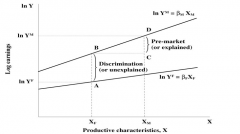
Oaxacca decomposition |
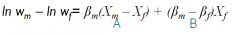
Decompose pay differential % -attributes -evaluation of attributes
|
|
|
Oaxacca decomposition graph |
|
|
|
Oaxacca decomposition limitation |
subject to omitted variable bias decomposition not unique corrective procedures developed |
|
|
Women differ because |
-Shorter market participation -higher turnover rate -absenteeism -household responsibilities |
|
|
Women choose |
-education -social work -soft people skill jobs Lower pay |
|
|
Combat discrimination policies |
-Conventional equal pay -Equal value, pay equity, comparable worth -Equal employment opportunity -Affirmative action/Employment equity -Facilitating policies |
|
|
Conventional equal pay |
within same job within same establishment |
|
|
Equal value, pay equity, or comparable worth |
between jobs of equal value -comparable worth has reduced the earning gap |
|
|
Equal employment opportunities |
may benefit new recruits |
|
|
Affirmative action/Employment equity |
Federal workers |
|
|
Equal pay across jobs |
- Generic factors ex.skills effort responsibility - Scaling - Levels with compensatable factors |
|
|
Policy initiatives impact |
-limited impact and scope -inconclusive |
|
|
Ethnic groups earning differentials |
-less evidence than female -measurement difficulty-immigrants |
|
|
women discrimination conclusions |
-wage diff between women and men, white and non-white -differences get small with characteristics -but discrimination may happen at market entry -not enough research for ethnic group |
|
|
Discrimination |
same ability inferior treatment |
|
|
Gender differences in human capital |
women less investment in human capital -take time out of labor force -benefits lost in earlier life -childbearing years are the highest return years -shorter worklife
|
|
|
Outcomes of gender gap |
-hs graduation -college -graduate -work experience |
|
|
wage gap and college major |
men in lucrative women in unlucrative |
|
|
gender diff in ed |
girls better in many men better in maths science |
|
|
sources of gender pay gap |
-diff occupations -within occupations earning gap still -gap small when controlled |
|
|
Immigration policy levers |
-number of admitted -Who is admitted |
|
|
immigration policy goals |
-max national welfare (skills) -evolve existing population (family unification) -humanitarian concerns |
|
|
Immigration classes |
- assessed - non-assessed |
|
|
Assessed |
-likely contribution and success -point system |
|
|
Non-assessed |
families and refuge |
|
|
Point system criterias |
Work experience Minimum funds Minimum score(educ, language, age, work exp, arranged emp) |
|
|
Impact of immigration on Employment and wages - supply only |
|
|
|
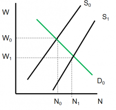
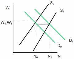
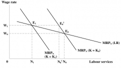
Impact of immigration on Employment and wages - supply and demand |
|
|
|
impact of immigration on consumers |
cheap labor -cheaper goods |
|
|
Impact of immigration on Employers |
greater profitability capital investment employment opportunities |
|
|
Immigration scale and substitution effect |
scale effect large enough to dominate substitution effect -complementary labor gains |
|
|
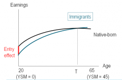
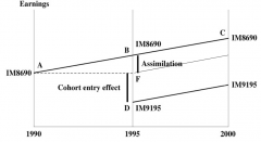
Entry effect |
immigrant suffer earning penalty -earnings rise over time -disparity can offset by short catch up period |
|
|
Assimilation profile |
|
|
|
Only assimilation effect, no entry effect |
|
|
|
Assimilation effect and no entry effect |
|
|
|
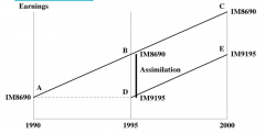
Empirical evidence on assimilation |
-entry effect worsening over time - return to education lower for immigrants - assimilation rates too low to catch up - |
|
|
US family reunification vs. Canada point system |
-point system reduces admission from less dev. countries -more skills -independent immigrants fare better |
|
|
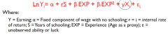
Wage depends on |
- education - work experience - Unobserved ability or luck - Other characteristics |
|
|
Earnings function |
|
|

|
|
|
|
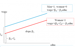
Why wage differentials |
Wages should be same across all regions - firms move to lower wage regions -workers move to higher wage regions -Mobility |
|
|
Effect of an oil shock on regional wages |
|
|
|
Reasons for wage differentials |
- compensating differentials - Immobility across sectors - Short run vs long run - Unobserved individual differences - non competitive factors |
|
|
Regional wage differentials |
- geographic preference - Compensating differences - non competitive factors |
|
|
Compensating differences |
cost of living remoteness climate pollution congestion |
|
|
Noncompetitive factors |
cost of moving artificial barriers policy barriers |
|
|
Interoccupational wage differential compensation for |
Nonpecuniary differences human capital investment endowed skills |
|
|
interoccupational wage differential Short Run adjustments |
demand for skilled labor |
|
|
Interoccupational noncomeptitive factors |
licensing unions legislations |
|
|
Interindustry wage differentials Non pecuniary aspects |
unpleasant/unsafe seasonal cyclinical |
|
|
Interindustry wage differential Short run demand factors |
reallocation technology changes free trade global competition |
|
|
Interindustry wage differential noncompetitve factors |
Monopoly rents unions licensing |
|
|
Offer above market wage to get |
-Improved morale -lower turnover -Discourage unionization -cost savings when not having to react to market changes |
|
|
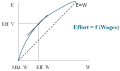
Efficiency wage theory |
higher wage means valued effort this value > cost of higher wages
|
|
|
Efficiency wage model |
|
|
|
Effort gain occured by |
-avoidence of shirking -unemployment creates incentive -reservation wage and selection |
|
|
Selection and reservation wages |
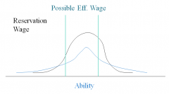
Higher wages attract higher ability workers |
|
|
Large firms are wage enhancing |
- unionized - Need more skilled workers - Monopoly rents shared with employees - Undesirable work conditions - use of efficiency wage to reduce monitoring - unobserved individual heterogenuity |
|
|
Human capital model and training |
-inc. worker productivity -initial costs and future returns - returns lost in separation |
|
|
Should the firm invest in training |
- Not if the skills are portable |
|
|
Should the worker invest in training |
-Not if the skills are firm-specific |
|
|
General training |
usable to all firms |
|
|
Specific training |
- usable only at the training firm |
|
|
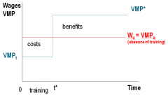
Cost benefit and financing of training -training absent |
|
|
|
When skills are transferable |
employees should bear cost -wages lower during training VMPt -after training employers offer market wage VMP* -training increases wage |
|
|
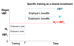
Training as shared investment |
|
|
|
Firm specific training but uncertainty about employment |
-wage premium to reduce turnover and recoup investment costs -lower the wage while training -shared costs and benefits |
|
|
Private markets training may not be socially optimal |
-imperfect information -regulations |
|
|
Government training subsidies |
increase working hours raise wages above the poverty line |
|
|
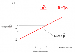
Regression line |
|
|
|
For every additional unit of variable s |
Log Y changes by beta unit. -dependent variable changes by beta unit variable |
|
|
Non linear effect regression |
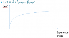
controlling for other variables |
|
|
Why use Wages in Ln |
-allows interpretation of parameter as % change -distribution of earning is skewed |
|
|
Why use Log for regression |
-pulls very large numbers and minimizes their diff. with other values -stretches out low values -better distribution |
|
|
Returns to education |
7-10% returns to an additional year of education -if pure experience then sum of % of earnings from each course -measurement issues & omitted ability bias |
|
|
Downward bias in education estimate |
-some not measured in higher wage -non-monetary benefits -creates attenuation bias |
|
|
Omitted Ability Bias |
- can't control for unobservable innate ability/talent ex.motivation
|
|
|
Additional Measurements of returns to education |
-Bachelors or masters relative to high school - field of study |
|
|
Compensating differenctials |
workers differ in preferences for job characteristics -firms differ in working conditions that they offer -match and mate in labor market |
|
|
Hedonic Wage model |
-Earning varies due to differences in nonpecuniary benefits - less pleasant conditions ex |
|
|
Hedonic wage model assumptions |
-Utility maximization -Worker information -Worker mobility |
|
|
Utility Maximization |
-compensating wage differentials occur if people prefer lower paying but more pleasant |
|
|
Worker information |
-workers aware of job characteristics of potential importance |
|
|
Workers mobility |
-range of job offers -employers offering dangerous work has to raise wages |
|
|
Employer's side |
Isoprofit schedule |
|
|
Isoprofit schedule |
combinations of wages and safety that firm can provide and maintain same level of profit -diminishing marginal rate of transformation between wages and safety |
|
|
Isoprofit schedule |
|
|
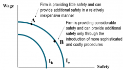
Different firms with different safety technologies |
-different abilities at given cost to provide safety -different isoprofit curves for different firms |
|
|
Different firms with different safety technologies |
|
|
|
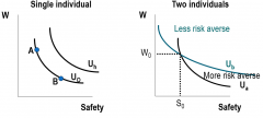
Individual's preference |
Iso-utility (indifference curve) may be willing to give up safety for compensating risk premium |
|
|
Worker indifference Curves |
|
|
|
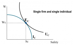
Equilibrium with Single Firm and a Single Individual |
Tangency between the iso-utility curve and isoprofit curve -Yields the optimal wage and safety |
|
|
Equilibrium with Single Firm and a Single Individual |
|
|
|
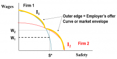
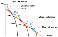
Equilibrium with many firms |
perfect competition -sort themselves into firms of different risks -compensating wages -wage safety locus |
|
|
wage-safety locus |
various equilibrium combinations of wages and safety |
|
|
Many firms and Many individuals |
|
|
|
Wage-Safety Locus |
Slope is negative -can change for different leves of safety -determined by preference and firms technology for safety |
|
|
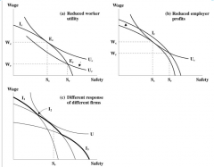
Effects of Safety Regulation |
Perfect information -safety regulations have no effect if already in safe jobs -lower the utility for high risk/wage jobs
|
|
|
Responses to Safety Standards |
|
|
|
Need for safety regulation |
-workers underestimate the risk -people are irrational -Negative externalities with worker injuries -worker compensation leads to accepting too much risk |
|
|
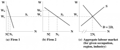
aggregate Labor Demand and Supply |
|
|
|
Unit payroll tax |
tax levied on employers proportional to firm's payroll often considered job killers |
|
|
Unit payroll tax examples |
CPP/QPP Worker's compensation Unemployment insurance Health insurance |
|
|
Effect of a Payroll tax on employment and wages is divided between employers and worker |
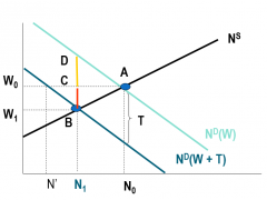
BC paid by workers |
|
|
Payroll Taxes effect |
depends on elasticity of labor |
|
|
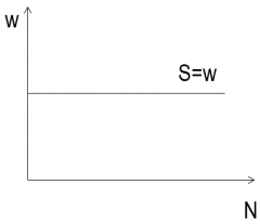
if inelastic supply(vertical S) |
no employment change -incidence of patroll tax falls largely on workers -disemployment effects small |
|
|
Monopsony |
Large firm relative to the size of labor market |
|
|
Monopsony hires more workers |
needs to raise wages |
|
|
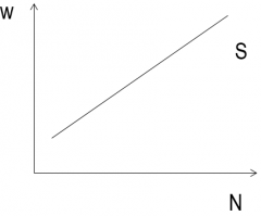
Monopsony Supply schedule |
upward sloping |
|
|
Monoposony if wages are decreased |
will not lose al workers |
|
|
Monopsony situations can happen |
-any firm in the short run -LR mobility costs -LR one industry town -LR very specialized |
|
|
Monopsony examples |
-nurse in a large hospital in small isolated town -mining company in small town -professional sports |
|
|
labour supply curve under perfect competition |
|
|
|
labour supply curve under monopsony |
|
|
|
profit maximization |
MRP=MC |
|
|
Monopsony profit maximization |
MC =/= w -doesn't take w as given
|
|
|
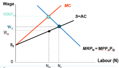
Monopsony hires an additional unit of labor |
must increase the wages paid to all workers |
|
|
Labour demand for monopsony |
|
|
|
Monopsony employment |
lower than in compteititve situation |
|
|
Monopsony employment restricted |
because hiring additional labor is costly |
|
|
Wage set by monopsonist |
lower than it would be if there was competition |
|
|
Sports owners |
small interconnected group can band together and act as monopsonist can set wages |
|
|
The greater is a league's monopsony power |
lower player salaries |
|
|
players will be paid |
below MRP |
|
|
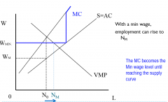
Minimum wages proponent |
Ensure a living wage make employment more attractive |
|
|
Minimum wages opponent |
increase unemployment minimum wage earners do not live in impoverished households |
|
|
Uniform coverage model |
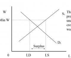
some unemployment created |
|
|
Monopsony minimum wage |
|
|
|
Short run |
Amount of capital fixed no SE |
|
|
Long run |
Capital varies response to wage change larger |
|
|
The demand for labor in the short and the long run |
|
|
|
Demand for labor decreases as |
wages increase -negative function |
|
|
wage increases |
adverse effect on employment |
|
|
Magnitude of the effect |
can be seen by elasticity of demand |
|
|
Elasticity of Demand |
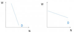
Measures the responsivesness of labor quantity
|
|
|
Elasticity of labor curve depends on |
size of substitution and scale effect |
|
|
Factors affecting Elasticity |
1.degree of substitution between factors of production 2. Elasticity of substitute input supply 3. Price elasticity of output demand 4. labour costs to total costs ratio |
|
|
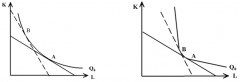
Degree of substitution between production factors |
|
|
|
The greater the degree of substitution between L and K |
flatter the labor demand curve greater wage elasticity of LR labor demand |
|
|
degree of factor substitution |
depends on state of technology unions |
|
|
If substitutes are relatively inelastic in supply |
If increasing demand drives up the price it may choke the usage |
|
|
Wage elasticity of labor demand |
depends on price elasticty of output demand |
|
|
labor demand |
derived demand |
|
|
Scale effect in labor demand |
depends on price elasticity of output demand |
|
|
increase in wage rate |
marginal cost cure rises |
|
|
if product demand very inelastic |
reduction in output very small very small scale effect on labor demand |
|
|
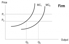
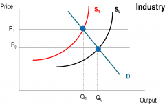
Cost increase on output |
|
|
|
If ratio of labor costs to toal costs is low |
increase in wage rate has small effect on total costs -> small scale effect -> labor demand curve very inelastic |
|
|
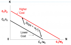
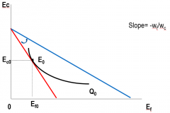
Outsourcing |
MRPnational=p*NPPnational MRPforeign=p*MPPforeign
Optimal condition: MPPnational/MPPforeign=Wnational/Wforeign |
|
|
Foreign and domestic labor |
tend to complement |
|
|
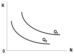
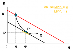
Isoquants |
Combinations of labor and capital used to produce a given amount of output -Marginal rate of technical substitution |
|
|
Isoquants |
|
|
Isocost Line |
All combinations of capital and labor that can be bought for a given total cost C= rK+ wN |
|
|
Isocost Line |
|
|
Cost-Minimizing |
|
|
|
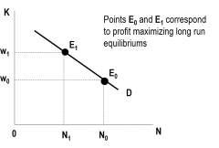
LR labor demand |
determined by LR profit maximizing labor requirements |
|
|
Effect of a Cost Increase on Output under perfect competition - firm |
|
|
|
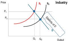
Effect of a Cost increase on output under perfect competition-industry |
|
|
|
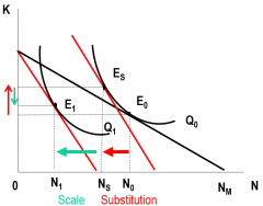
Substitution effect |
firm substitutes cheaper inputs for more expensive labor |
|
|
Scale effect |
Firm would reduce its scale of operations because of the cost increase associated with the increase in wage |
|
|
Wage Increase on labor demand |
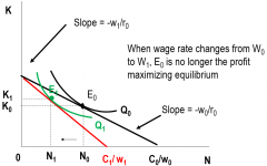
only substitution effect |
|
|
wage increase with substitution and scale effect |
|
|
|
Derived LR Labor demand schedule |
|
|
|
If foreign wages drop while outsourcing -close substitutes |
|
|
|
If foreign wages drop while outsourcing -low degree of substitution |

|
|
|
Demand for labor |
derived by output produced by firm |
|
|
Firm objective |
Profit maximization |
|
|
Firm constraints |
-market structure - Demand for the product - Factor prices - Production function(maximum output) - Decision making time frame(SR/LR) |
|
|
Production function assumptions |
Labor (N) Capital (K) - fixed in SR produce (Q)
|
|
|
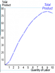
Total product |
Total product produced using given combination |
|
|
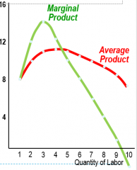
Average product |
APn =TP/N |
|
|
Marginal product of labor |
Additional output produced with one additional unit of labor |
|
|
Law of diminishing returns |
|
|
|
Marginal Product and average product |
|
|
|
Costs |
- Fixed ( sunk cost) - Variable |
|
|
Decision Rule 1 |
Operate as long as variable costs are covered TR=TVC |
|
|
DEcision Rule 2 (competitive) |
MC = MR which is wage = p |
|
|
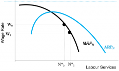
Marginal revenue product of labor |
MRPn - extra revenue generated by selling one additional unit that can be attributed to labor = MR * MPn which is = p * MPn |
|
|
Decision rule for employment |
Hire to MRPn=MCn MRPn > MCn increase employment MRPn < MCn decrease employment - Increase MCn til MRPn=MCn |
|
|
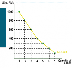
Characteristics of a firm in a competitive market |
- price taker - can hire labor w/o impacting market wage - MC= w - Hire until MRP = w (MC) - SR labor demand curve is MRP curve |
|
|
SR demand for labor |
|
|
|
MRP is a labor demand curve because |
firm only hires worker if it adds more to revenues than it adds to wage costs -slopes down |
|
|
SR labor demand
|
|
|
|
SR labor demand |
downward sloping because of diminishing marginal returns to labor -wage down demand up
|