Reading...
![]()
Play button
![]()
Play button
![]()
Use LEFT and RIGHT arrow keys to navigate between flashcards;
Use UP and DOWN arrow keys to flip the card;
H to show hint;
A reads text to speech;
48 Cards in this Set
- Front
- Back
- 3rd side (hint)
|
compare the mean of a single sample with the population mean proposed in a null hypothesis
|
one-sample t-test
|
H0: The true mean equals µ0.
HA: The true mean does not equal µ0. |
|
|
df for one-sample t-test
|
df = number of independent data points - 1
|
|
|
|
µ
|
Population Parameter − a quantity describing a population (truth)
|
|
|
|
Precision
|
the spread of estimates resulting from sampling error.
|
|
|
|
Bias
|
systematic discrepancy between estimates and the true population characteristics.
|
|
|
|
Random sample
|
each member of a population has an equal and independent chance of being selected.
|
|
|
|
the different categories have no inherent order
|
Nominal Categorical
|
|
|
|
variables that can be ordered, despite lacking magnitude on the numerical scale.
|
Categorical Ordinal
|
|
|
|
can take on any real-number value within some range
|
Numerical Continuous
|
|
|
|
numerical data with indivisible units
|
Numerical Discrete
|
|
|
|
Experimental study
|
the researcher assigns different treatment groups or values of an explanatory variable randomly to the individual units of study.
|
|
|
|
Observational study
|
the assignment of treatments is not made by the researcher.
|
|
|
|
graph categorical data
|
Bar graph
|
|
|
|
graph numerical data
|
Histogram
Cumulative frequency distribution |
|
|
|
graph two categorical variables
|
Grouped bar graph
Mosaic plot |
|
|
|
graph one numerical variable and one categorical variable
|
Grouped histogram
Cumulative frequency distribution Line plot (ordinal categories only) |
|
|
|
First quartile
|
the middle value (median) of the measurements lying below the median.
|
|
|
|
Second quartile
|
the median
|
|
|
|
Third quartile
|
the middle value (median) of the measurements larger than the median.
|
|
|
|
Extreme values
|
those lying farther from the box edge than 1.5 times the interquartile range; displayed by dots.
|
|
|
|
Proportion
|
most important descriptive statistic for a categorical variable.
p-hat = number in a category/n |
|
|
|
95% confidence interval for the mean
|
We are 95% confident that the population mean falls between ____ and ____.
|
|
|
|
2SE Rule of Thumb
|
A rough approximation to the 95% confidence interval for a mean can be found from the sample mean plus and minus two standard errors.
|
|
|
|
Addition rule
|
if two events A and B are mutually exclusive, then Pr[A or B] = Pr[A] + Pr[B]
|
|
|
|
Generalized addition rule
|
works for both mutually exclusive and not mutually exclusive events.Pr[A or B] = Pr[A] + Pr[B] - Pr[A and B]
|
|
|
|
Multiplication rule
|
if two events A and B are independent, then Pr[A and B] = Pr[A] x Pr[B]
|
|
|
|
General multiplication rule
|
finds the probability that both of two events occur, even if the two are dependent.
Pr[A and B] = Pr[A] Pr[B|A] |
|
|
|
Law of total probability
|
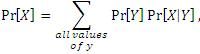
|
Example:
Pr[egg is male] = Pr[host already parasitized] x Pr[egg is male|host already parasitized] + Pr[host not parasitized]Pr[egg is male|host not parasitized] = (0.2 x 0.9) + (0.80 x 0.05) = 0.22 |
|
|
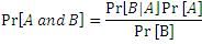
Baye's theorem
|
|
|
|
|
Type I error
|
rejecting a true null hypothesis
|
|
|
|
Type II error
|
failing to reject a false null hypothesis
|
|
|
|
binomial distribution assumptions
|
The number of trials (n) is fixed. Separate trials are independent. The probability of success (p) is the same in every trial.
|
|
|
|
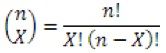
n choose X
|
|
|
|
|
test whether a population proportion (p) matches a null expectation(p0) for the proportion.
|
Binomial test
|
H0: The relative frequency of successes in the population is p0.
HA: The relative frequency of successes in the population is not p0. |
|
|
test statistic for binomial test
|
observed number of successes
|
|
|
|
Adjusted Wald Method
|
used to calculate an approximate confidence interval for a proportion.
|
|
|
|
measures the discrepancy between an observed frequency distribution and the frequencies expected under a simple random model serving as the null hypothesis.
|
X2 Goodness-of-Fit Test
|
|
|
|
Degrees of Freedom for X2
|
df = (number of categories) − 1 − (number of parameters estimated from the data)
|
|
|
|
X2 Specific Assumptions
|
None of the categories should have an expected frequency less than one.
No more than 20% of the categories should have expected frequencies less than five. |
|
|
|
probability of getting X successes in a block of time or space, when successes happen independently of each other and occur with equal probability at every point in time or space.
|
Poisson Distribution
|
|
|
|
Degrees of Freedom for Poisson
|
df = number of categories - 1 - 1
|
|
|
|
variance is greater than the mean
|
distribution is clumped
|
|
|
|
variance is less than the mean
|
distribution is dispersed
|
|
|
|
estimates and tests for an association between two or more categorical variables.
|
X2 contingency test
|
H0: categorical variable 1 and 2 are independent.
HA: categorical variable 1 and 2 are not independent. |
|
|
degrees of freedom for the X2 contingency test
|
df = (r-1)(c-1)
|
|
|
|
Standard normal distribution
|
a normal distribution with mean 0 and standard deviation 1.
|
|
|
|
Student's t
|
the difference between the sample mean and the true mean (Y̅ − µ), divided by the estimated standard error (SEY̅)
|
|
|
|
coefficient of variation
|
CV = 100% (standard deviation/mean)
|
|