![]()
![]()
![]()
Use LEFT and RIGHT arrow keys to navigate between flashcards;
Use UP and DOWN arrow keys to flip the card;
H to show hint;
A reads text to speech;
31 Cards in this Set
- Front
- Back
|
Ensemble Modeling Fundamentals |
Ensemble modeling aims at forecasting a given response variable with higher accuracy compared to an individual prediction model. To that end, the forecasts of a collection of prediction models, which show some synergy and complement each other, are pooled to produce a composite
forecast. |
|
|
General Functioning of Ensemble Models |
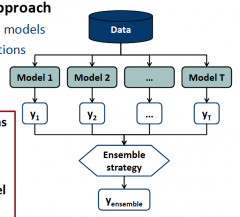
Multi‐step modeling approach Develop a set of (base) models
Aggregate their predictions
Several ensemble algorithms have been proposed. These algorithms differ mainly in how they develop base models and pool base model
predictions, respectively.
|
|
|
Why Forecast Combination Increases Accuracy |
Different methods have different views on the same data For example linear versus nonlinear models Forecast combination gathers information from multiple sources Like asking many experts for their opinion Formal explanation Bias‐variance‐trade‐off Strength‐diversity‐trade‐off Ensemble margin Much empirical evidence Forecasting benchmarks in various domains Credit scoring, insolvency prediction, direct marketing, fraud detection,
project effort estimation, software defect prediction, and many others |
|
|
Ensembles and the Bias‐Variance‐Trade‐Off |
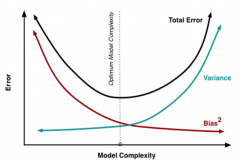
Bias and variance reduce predictive accuracy Complex classifiers Low bias High variance Simple classifiers High bias
Low variance |
|
|
Ensembles and the Strength‐Diversity Trade‐Off |
The success of an ensemble depends on two factors: the strength of and the diversity among the base models. Base model strength How well they forecast future cases Predictive accuracy Base model diversity Extent to which base model predictions agree Can think of diversity as forecast (or error) correlation Research on strength‐diversity trade‐off focuses on
ensemble classifiers
There is no point in combining identical models. If all base models in an ensemble make the same predictions,
combination cannot increase accuracy.
Imagine a perfect model Always predicts with 100% accuracy Maximal strength Put this model into an ensemble Average of perfect prediction with other predictions No way to increase accuracy Implication: Since all classifiers predict the same target, they cannot be very strong and highly diverse at the same time. There is a conflict
between strength and diversity.
|
|
|
Diversity in Classifier Ensembles |
Different classifier outputs require different measures Estimates of posterior class probabilities (numeric) Estimates of class membership (discrete) Motivates research associated with Developing diversity measures Studying the behavior/features of different measures Exploring the extent to which diversity explains ensemble success Examining whether diversity maximization is a good idea Till now, no consensus on any of these questions Key take‐away: Understanding diversity is useful to understand different types of
ensemble classifiers.
Categories of diversity measures Pairwise (e.g., Q‐statistic, correlation, disagreement, doublefault measure, etc.) Non‐pairwise (e.g., entropy, Kohavi‐Wolpert variance,
generalized diversity, etc.) |
|
|
Strength‐Diversity‐Plots |
The distribution of base classifier strength and diversity
is often illustrated by means of a scatter plot. |
|
|
Ensemble Margin Exemplified |
Several studies have shown that the generalization performance of an ensemble is related to the distribution of its margin on the training sample. The larger the margin the better
Generalization error upper‐bounded by ensemble margin |
|
|
Homogeneous Ensemble Classifiers |
Produce base models using the same algorithm Inject diversity through manipulating the training data Drawing training cases at random (e.g., Bagging)
Drawing variables at random (e.g., Random Subspace) |
|
|
Heterogeneous Ensemble Classifiers |
Produce base models using different algorithms Inject diversity algorithmically Different classification algorithms Different meta‐parameter settings per classification algorithm Also called multiple‐classifier‐systems 20‐Oct‐14 Business Analytics & Predictive Modeling, Chapter 8, Stefan Lessmann 22 Heterogeneous Ensemble Classifiers
Ensemble |
|
|
Ensemble Classifiers Without Pruning |
Two‐step approach Develop base models (homogeneous or heterogeneous) Put all base models into the ensemble
Standard practice |
|
|
Ensemble Classifiers With Pruning |
Three‐step approach Develop candidate base models (typically heterogeneous) Optimize ensemble composition using some search strategy Put selected base models into the ensemble; discard the rest Active field of research Which search strategy?
Which objective? |
|
|
Homogeneous Ensemble Algorithms |
Bagging Random Forest
Boosting |
|
|
Bagging |
Given a classification algorithm, bagging derives base models from bootstrap samples of the training set. Bootstrap sampling Given data set of size n
Draw random sample of size n with replacement |
|
|
A Note on Bootstrapping |
bootstrap sample includes some cases multiple times About 37% of the original cases do not appear at all Called out‐of‐bag (OOB) examples Facilitate assessing a model on hold‐out data
Facilitate assessing variable importance |
|
|
Base Model Combination |
Every bootstrap sample provides one base model Predictions are combined using majority voting Typical formulation used in textbooks Can be misleading Classifiers produce different types of predictions Binary class predictions Numeric confidences (magnitude of values indicate likelihood of class)
Class probabilities (e.g., p(y=1|x)) |
|
|
Bagging and the Bias‐Variance‐Trade‐Off |
Bias Depends on the base classifier Not altered due to bagging Variance Reduced due to combining base models from different bootstrap samples As in any ensemble model
Bagging increases predictive accuracy through reducing variance. |
|
|
Tuning a Bagging Classifier |
Meta‐parameters of bagging Classification algorithm Preferably tree‐based or neural network But can use any Could also tune meta‐parameters of the (base) classifier How many bootstrap samples (i.e., ensemble size) Size of bootstrap sample Often overlooked but useful when working with large data sets Practical advice: The larger the ensemble the better. Given data and resources,
develop the largest bagging ensemble possible. |
|
|
Bagging Assessed |

|
|
|
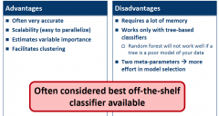
Random Forest |
Combines bagging with random subspace Improves approach to inject diversity “Forest” = collection of “trees”
Works only with tree‐based classifiers Grow each tree from a bootstrap sample of the training data (exactly as bagging) In addition, When choosing an attribute to split the data Do not search among all attributes Instead, draw random sample of attributes (Random Subspace) Find best split from attributes within sample Increased diversity Random subspace limits access to attributes Forces tree‐growing algorithm to explore different ways to
separate the data |
|
|
Random Forest and the Bias‐Variance‐Trade‐Off |
Tree‐based classifiers tend to overfit the data Always possible to perfectly separate your data Just find as many rules as there are cases in your data Pruning is a way to avoid overfitting Breiman recommends to not prune decision trees Fully‐grown decision trees (without pruning) Have zero bias (by definition) Have high variance Bootstrapping many such decision trees reduces variance Random forest increases predictive accuracy through using classifiers without
bias while avoiding the problem of high variance through bootstrapping. |
|
|
Tuning a Random Forest Classifier |
Meta‐parameters of random forest Size of the random sample of attributes (often called mtry) Forest size (number of bootstrap samples) Size of bootstrap sample
Often overlooked but very useful when working with large data sets |
|
|
Random Forest Assessed |
|
|
|
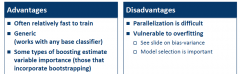
Boosting |
General idea It is often easy to find a simple classifier If AGE < 25 Then RISK = High Finding many such simple classifiers is easier than finding one very powerful classifier Combining many simple classifiers also gives a powerful classifier Note:
Simple classifiers are called weak learners in the boosting literature. |
|
|
Base Model Development |
Basic idea Develop one (simple) classifier Check which cases it gets right and which cases it gets wrong Develop second classifier that corrects the errors of classifier 1 Check errors of the ensemble (classifier 1 + classifier 2) Develop third classifier that corrects the errors of the ensemble
Repeat
It is common that the weights of base classifiers vary a lot. Classifiers with large absolute weight have a big impact on the ensemble prediction. Basically, the weight of a classifier depends on its accuracy. However, the weight also takes into account, how difficult it was to classify a specific case correctly. This way, classifiers that do not contribute new information receive low
weights.
|
|
|
Boosting and the Bias‐Variance‐Trade‐Off |
Prevailing view is that boosting reduces bias and
variance
Given that the ensemble is large enough, training error and thus bias
reduces to zero. |
|
|
Tuning a Boosting Classifier |
Meta‐parameters of boosting Classification algorithm for base model construction Often shallow decision trees (sometimes called decision stumps) Embody idea to use weak classifier Use of other base classifiers is possible (depending on software package) How many iterations (i.e., ensemble size) Maybe more meta‐parameters Depending on boosting implementation and software package Practical advice: There is little need to try different base classifiers. Trees work fine in most applications. Apply model selection to determine no. of iterations. Suggestion: try sizes of 10, 25, 50, 100, 250, 500. You can use larger settings as well but note that
training time will increase. Consider gbm package when using R. |
|
|
Boosting Assessed |
|
|
|
Multiple Classifier Systems |
A multiple classifier system is an ensemble in which the base models are produced using different classification algorithms. Active field of research Which factors determine the success of a MSC? How to weight base classifiers? Use all base models or optimize MCS composition? The simplest MCS possible Build a collection of base models using your preferred classification algorithms and compute the simple average over
their predictions.
Discrete class prediction Continuous confidences Class probabilities Averaging requires predictions of a common scale Recommendations Avoid classifiers that produce discrete class predictions only
Calibrate base classifier predictions |
|
|
Final Note on Stacking |
Predictions of base classifiers are highly correlated All base classifiers predict the same response variable Use robust classifier for 2nd level Classic statistical classifiers suffer from multicollinearity Avoid such classifiers (logistic regression, discriminant analysis, etc.) Modeling process gets very complex when 2nd level classifier requires model selection Which data to use for parameter tuning? Avoid classifiers with many meta‐parameters and/or classifiers that are sensitive to meta‐parameter choice In view of the above Option 1: Regularized logistic regression (try = 100)
Option 2: Random forest using rule of thumb for mtry |
|
|
Multiple Classifier Systems Assessed |

|