Reading...
![]()
Play button
![]()
Play button
![]()
Use LEFT and RIGHT arrow keys to navigate between flashcards;
Use UP and DOWN arrow keys to flip the card;
H to show hint;
A reads text to speech;
86 Cards in this Set
- Front
- Back
|
Central Limit Theorem
|
For populations that aren’t normally
distributed, if n ≥ 25, X ̄ approx. ∼ N(μ,σ2/n). |
|
|
significance level
|
aka Type I error rate
if H0 true, when # tests -> infinity, % of tests rejected under alpha by chance -> 5 percent |
|
|
cor(X, Y )
|
cov(X, Y )/σX σY
|
|
|
cor(X, Y ) = 0 =⇒??
|
ONLY IF X, Y ~N, X, Y are independent
|
|
|
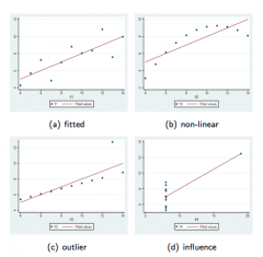
Four Kinds of Influence
|
|
|
|
Reversability of correlation
|
Cor(X,Y) = Cor(Y,X)
|
|
|
Error term in Simple Regression
|
assumed mean/E(epsilon-i) = 0, variance constant, epsilon-i and epsilon-j uncorrelated so covariance is zero for all i, j i=/j
|
|
|
Adjectives for regression models and what they mean
|
simple = one predictor
'linear in the parameters' = no paramater appears as exponent or multiplied/divided by other parameter (nonlinear) |
|
|
Yi (response variable) -- random?
|
Yes: random error term added makes Yi a random var
|
|
|
E(Yi)
|
Since E(error-i) = 0, E(Yi) = Beta0 + Beta1*(Xi)
so predicted model is E(Y|X) = Beta0 + Beta1*(X) |
|
|
Distribution of Yi
|
Since errors are (are assumed) to be normally distributed N(0, sigma^2),
Yi ~ N(Beta0 + Beta1(Xi), sigma^2) |
|
|
Predicting changes in Y when X changes
|
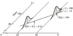
Beta0 and Beta1 describe the relationship between the *mean* of Y and X, while the variance of the residuals sigma^2 describes variability of Yi around the mean
|
|
|
Beta0 and Beta1 in terms of E(Y)
|
E(Y|X=0) = Beta0
E(Y|X=x+1) - E(Y|X=x) = Beta1 |
|
|
Ordinary Least Squares regression
|
a way to find Betas; minimizes the sum of squared residuals, where residual ei = Yi - Yhat (i.e. solves calculus minimization for sum of squared residuals Sigma[(Yi - Beta0 - Beta1*Xi)^2] )
|
|
|
Three Assumptions of LS Regression
|
All observations are uncorrelated:
- corr(Yi, Yj) = corr(error-i, error-j) = 0 All observations are equally informative: - Var(Yi) = Var(error-i) = sigma^2 There is no systematic bias in the model E(error-i) = 0 For testing & inference, fourth assumption is that errors are ~ N(0, sigma^2) |
|
|
Least Square regression estimate of B1
|
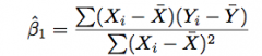
E(Beta1-hat) = Beta1;
var(Beta1-hat) = sigma^2/Sigma[(Xi - Xbar-i)^2] |
|
|
Least Square regression estimate of B0
|
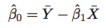
E(Beta0-hat) = Beta0
|
|
|
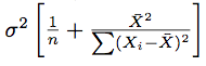
B0-hat Variance
|
|
|
|
B0hat and B1hat distributions
|
Because sigma^2 (of Yi and error-i) isn't known, distributed t with n-2 degrees of freedom
|
|
|
Consequences of LS assumptions
|
Sum of residuals is 0, Sum of observations = sum of fitted values (Sigma(Yi) = Sigma(Yhat-i), regression line always goes through (Xbar, Ybar)
|
|
|
Why least squares estimators are random variables
|
different samples yield different values !
|
|
|
Distribution of least square estimators & associated test statistic
|
if errors are normally distributed as assumed, they are normally distributed;
For testing H0: Beta = 0eta-hat - 0 / S.e.(Beta-hat) ~ N or t(n-2) depending on sample size |
|
|
"Is there a relationship between...?"
|
First look at correlation to determine if vars are linearly related and if so what direction relationship is in -- can also just look at a scatterplot to glean this. To quantify the relationship we employ SLR (simple linear regression) and look at R^2, which is the square of the correlation coefficient between X and Y (for simple linear regression).
|
|
|
What R^2 is and means
|
R^2 is the amount of variation in response that can be explained by predictor(s) in model ALONE, ignoring the effect of other things not in model; R^2 = SSR/SST
R^2 is NOT GOOD FOR TESTING, only for understanding. |
|
|
Bonferroni correction
|
Testing both hypotheses at once requires adjustment to the significance level of each in order to preserve the overall significance level of the entire test
If k tests are performed, at least one of them needs to be significant at alpha/k for overall testing to be signficiant |
|
|
Standard error for mean response (prediction)
|
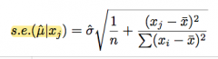
note smaller than forecast because it's harder to estimate a single point; "standard error of the fitted value"
|
|
|
Standard error for one observation (forecast)
|
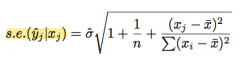
"standard error of the forecast value"
Forecast interval is technically NOT a confidence interval. It is not for testing! This is a 95% highest probability density interval for the new forecast variable. |
|
|
Graphical interpretation of Betas in MLR
|
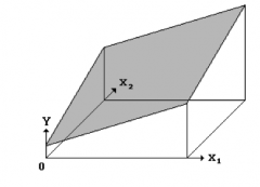
Beta1 = effect of X1 on Yhat with all other predictors held constant ('adjusted for other Xs')
|
|
|
Collinearity
|
inter-predictor relationship
|
|
|
An example of model fitting procedure
|
1) look at scatter matrix, check out which predictors have a clearly linear relation to outcome
2) |
|
|
Comparing R^2 of regress y x1 and regress y x2 to R^2 of regress y x1 x2
|
Rcombined^2 <= R1^2 + R2^2; only equal if X1 and X2 are totally unrelated
|
|
|
Deriving betas for regress y x1 x2 from regress y x1 and regress y x2
|
To find the unique contribution of x2 that is not already explained by x1, we regress the unexplained part of y onto the unexplained part of x2. We use **eyx1∼ex2x1**. Beta1 from this regression is x2's regression coefficient.
|
|
|
Marginal vs. partial coefficients
|
marginal coefficient Beta1 in SLR describes effect of X1 on Y ignoring all other variables; partial coefficient Beta1 in MLR describes effect of X1 on Y 'adjusted for' other predictors (i.e. with other predictors fixed).
|
|
|
Difference in distribution of predictors for MLR
|
All holds as in SLR, but estimates are distributed on t- with n-p-1 degrees of freedom. Residual variance still estimated with s^2.
|
|
|
How to test H0: all coefficients are zero
|
1) compare p-values associated with each Beta to alpha/(# parameters); if at least one exceeds significance can reject H0
OR 2) Cf. Overall F-test in regression output w/ associated p-value; this p-value is defaulted to be a measure of extremity against your H0 |
|
|
How to test H0: some coefficients are zero
|
1) Bonferroni
2) Run FM (full model) and RM (reduced model) regressions and compare adjusted R^2 (adjusts for # parameters) 3) Partial F-test ('exact' way) |
|
|
Adjusted R^2
|
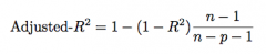
unlike R2, adjusted R2 has expectation zero, and it can be negative
|
|
|
Partial F-test
|
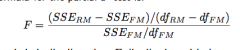
df of distribution is difference in # of parameters in two models and n-p-1 (df of full model)
judiciously, can be used for the following scenarios: Testing whether one single coefficient is 0, Testing whether all coefficients are simultaneously 0, Testing whether several coefficients are simultaneously 0 |
|
|
Testing H0: Beta1=Beta2
|
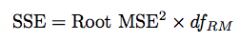
Two ways to do this; first way is to generate a new variable Star = X1+X2
If full model is, for example: Y = Beta0 + Beta1X1 + Beta2X2 reduced model to compare is Y = Beta0 + Beta1(X1+X2 = Star) Alternatively, can derive SSE of reduced model from Root MSE which is on output of 'constrain', and can calculate partial F-statistic from there. |
|
|
Implications of Unmet Assumptions
|
for example: If errors are not ~N, least square estimates don't have known distribution, can't test hypotheses b/c statistics are undefined
|
|
|
Implications of Unmet Assumptions
|
for example: If errors are not ~N, least square estimates don't have known distribution, can't test hypotheses b/c statistics are undefined
|
|
|
Implications of Unmet Assumptions
|
for example: If errors are not ~N, least square estimates don't have known distribution, can't test hypotheses b/c statistics are undefined
|
|
|
Implications of Unmet Assumptions
|
for example: If errors are not ~N, least square estimates don't have known distribution, can't test hypotheses b/c statistics are undefined
|
|
|
Main assumption of regression inference
|
Errors are iid ~ N(0,Sigma^2)
|
|
|
Main assumption of regression inference
|
Errors are iid ~ N(0,Sigma^2)
|
|
|
Main assumption of regression inference
|
Errors are iid ~ N(0,Sigma^2)
|
|
|
Main assumption of regression inference
|
Errors are iid ~ N(0,Sigma^2)
|
|
|
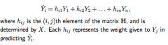
Leverage
|

hii, the amount of weight Yi is given in predicting Yhat-i, is the leverage of the i-th observation
|
|
|
Leverage
|

hii, the amount of weight Yi is given in predicting Yhat-i, is the leverage of the i-th observation
|
|
|
Leverage
|
hii, the amount of weight Yi is given in predicting Yhat-i, is the leverage of the i-th observation
|
|
|
Leverage
|

hii, the amount of weight Yi is given in predicting Yhat-i, is the leverage of the i-th observation
|
|
|
About Variance of Residuals and Why its the case
|
although residuals do have mean 0, but each has different variance. In addition, they are correlated
because looking at Yhat-i in terms of leverage, we see that all residuals are estimated from the same data, and they each interdepend on the rest of the observations |
|
|
Leverage point
|
if hii (leverage) is close to 1; means that Yi plays a strong role in predicting Yhat-i; means further that Yi is an outlier
|
|
|
Leverage point
|
if hii (leverage) is close to 1; means that Yi plays a strong role in predicting Yhat-i; means further that Yi is an outlier
|
|
|
Leverage point
|
if hii (leverage) is close to 1; means that Yi plays a strong role in predicting Yhat-i; means further that Yi is an outlier
|
|
|
Leverage point
|
if hii (leverage) is close to 1; means that Yi plays a strong role in predicting Yhat-i; means further that Yi is an outlier
|
|
|
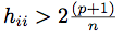
Screen for leverage points
|

|
|
|
Screen for leverage points
|
|
|
|
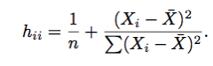
Leverage in SLR
|
|
|
|
Leverage in SLR
|

|
|
|
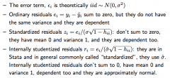
standardized residual
|
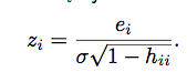
mean 0, variance 1; note that this relies on Sigma (variation of error) which is infrequently known (IE THESE ARE RARE!)
|
|
|
standardized residual
|

mean 0, variance 1; note that this relies on Sigma (variation of error) which is infrequently known (IE THESE ARE RARE!)
|
|
|
studentized residual
|
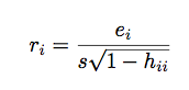
s is estimate of Sigma
in STATA: rstandard = studentized (our class) = 'internally studentized' (the book) "too big" is > 2, and these residuals no longer add up to 0 |
|
|
studentized residual
|

s is estimate of Sigma
in STATA: rstandard = studentized (our class) = 'internally studentized' (the book) "too big" is > 2, and these residuals no longer add up to 0 |
|
|
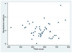
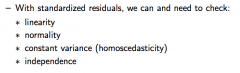
Checking Homoscedacity with Studentized residuals
|

rstandard vs fitted values 'box of judgement'
|
|
|
Checking Homoscedacity with Studentized residuals
|

rstandard vs fitted values 'box of judgement'
|
|
|
Checking normality with studentized residuals
|

Q-Q plot!
|
|
|
Checking normality with studentized residuals
|
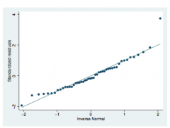
Q-Q plot!
|
|
|
Checking linearity with studentized residuals
|

rstandard vs fitted values scatter
|
|
|
Checking linearity with studentized residuals
|
rstandard vs fitted values scatter
|
|
|
Checking independence with studentized residuals
|

Only pertinent if order matters in data; index plot of rstandard
|
|
|
Checking independence with studentized residuals
|

Only pertinent if order matters in data; index plot of rstandard
|
|
|
I decided to omit a predictor from my model. How do I check if this omitted content is correlated with my new model's residuals?
|
scatter plot of residuals vs omitted predictor; if you see a linear pattern you should see if adding the variable back in is a benefit!
|
|
|
I decided to omit a predictor from my model. How do I check if this omitted content is correlated with my new model's residuals?
|
scatter plot of residuals vs omitted predictor; if you see a linear pattern you should see if adding the variable back in is a benefit!
|
|
|
Review Placard
|
|
|
|
Review Placard
|

|
|
|
Review placard contd
|
|
|
|
Insidious Outliers!
|
outlier(s) --> big residual --> overstated s.e. --> internally studentized residuals are too SMALL --> ability to detect less glaring outliers and to check assumptions is impaired
EXTERNALLY STUDENTIZED residuals conceived in response -- these are from MSE, which don't need the whole data (can leave out outliers to make a more 'usual' data set) |
|
|
externally studentized or 'jackknife' procedure
|

dont want to contaminate w obs that will be dropped later, so calculate s.e. w/o current obs
tends to make outlier residuals more prominent than internally studentized residuals |
|
|
Potential harm of keeping an outlier
|
regression surface tilted to accommodate them, OR if MSE inflated too much. This extra noisiness could mask other
outliers and/or regression violations |
|
|
Potential harm of dropping an outlier
|
may introduce bias!
|
|
|
Influence
|
a point is influential if removing the point causes substantial model change
In order to have much influence, a case must have large leverage AND residual |
|
|
Cook's Distance
|
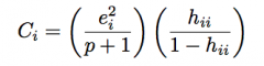
Residual^2 * potential
Cook’s distance combines the size of the residuals with the amount of leverage. Both are required to be large for Cook’s distance to be large. Large Cook’s distance means likely outlier and likely leverage point (i.e. likely influence point). |