Aggregate Supply And Aggregate Demand

Front 1

What is the AS-AD model?

Back 1

The AS-AD model is a model of an imaginary market for the total of all the final goods and services.

The ‘quantity’ is real GDP and he ‘price’ is the price level measured by the GDP deflator.

Front 2

What is quantity of real GDP supplied?

Back 2

The total quantity of goods and services, valued in constant base year, that firms plan to produce during a given period. It depends on labour supply and labour productivity.

Front 3

What is aggregate supply?

Back 3

The relationship between the real GDP supplied and the price level, and differs in the long and short run.

Over the business cycle, employment fluctuates around full employment, and the quantity of real GDP supplied fluctuates around potential GDP.

Front 4

What is long run aggregate supply?

Back 4

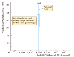
The relationship between the quantity of real GDP supplied and the price level when the money wage rate changes in step with the price level to maintain full employment. The curve is called 𝐿𝐴𝑆.

The quantity of real GDP supplied at full employment = potential GDP (independent of price level).

𝐿𝐴𝑆 is vertical at potential GDP, because a movement along the curve is accompanied by a change in two sets of prices – The price of goods and services (price level), and prices of factors of production (money wage rate).

A change in the price level means money wage rate increases by the same amount, and the real wage rate remains the same. Therefore, employment remains constant and real GDP remains constant at potential GDP.

Front 5

Long-run aggregate supply

Back 5

Front 6

What is short run aggregate supply?

Back 6

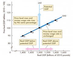
The relationship between the quantity of real GDP supplied and the price level when the money wage rate, the prices of other resources and potential GDP remain constant. The curve is 𝑆𝐴𝑆.

In the short run, an increase in the price level brings an increase in the quantity of real GDP supplied.

𝑆𝐴𝑆 is sloping upward.

Since the money wage rate is given, the price level when real wage rate is at full-employment equilibrium level is when 𝑆𝐴𝑆 = 𝐿𝐴𝑆.

Front 7

Short-run aggregate supply

Back 7

Front 8

Describe changes in potential gdp

Back 8

When potential GDP increases, 𝐿𝐴𝑆 and 𝑆𝐴𝑆 shift to the right. Both curves shift by the same amount only if the full employment price level remains constant (assumed in this case).

Potential GDP increases due to:

Increase in full-employment quantity of labour – Real GDP increases as the labour force increases.

Increase in quantity of capital (human and physical) – The workforce becomes more productive.

Advance in technology – Firms produce more, even with fixed quantities of labour and capital.

Front 9

Changes in money wage rate and other resource prices

Back 9

𝑆𝐴𝑆 changes and 𝐿𝐴𝑆 does not.

A rise in the money wage rate and resource prices means 𝑆𝐴𝑆 shifts leftward, because they increase firms’ costs.

Firms are therefore willing to reduce production at any given price level.

The changes would not affect the 𝐿𝐴𝑆, since a change in the money wage rate is accompanied by an equal percentage change in the price level (same money wage and price level rise in the long run). Therefore, real wages and production costs remain unchanged.

The money wage rate changes due to: Departures from full employment – Above-natural unemployment rate puts downward pressure on money wage rate and vice versa. Expectations about inflation – Money wage rate rises faster with expected increase in inflation rate and vice versa.

Front 10

Define: Quantity of real GDP demanded

Back 10

The total amount of final goods and services produced in the UK that people, businesses, governments and foreigners plan to buy. I.e. the sum of consumption expenditure, investment, government expenditure, and net exports: 𝑌 = 𝐶 + 𝐼 + 𝐺 + 𝑋 − 𝑀

Front 11

Define: Aggregate demand

Back 11

The relationship between the quantity of real GDP demanded and the price level. The buying plans which sum up to get AD depend on:

The price level

Expectations

Fiscal and monetary policy

The state of the world economy.

Front 12

Describe the aggregate demand curve

Back 12

The aggregate demand curve, 𝐴𝐸, slopes downwards because of the wealth and substitution effect.

Front 13

What is the wealth effect?

Back 13

Other things being equal, a rise in the price level decreases quantity of real wealth because consumers hold nominal assets.

Real wealth is amount of money in the bank, bonds, shares and other assets that people own (not measured in pounds).

People save and hold real wealth for multiple reasons (mainly to provide retirement income).

Consumers may save more in order to restore real wealth to its original level. Others accept the new level.

For both groups, planned consumption falls

Front 14

What is the substitution effect?

Back 14

Other things being equal, a rise in the price level means real amount of money in the economy falls, so banks have less money to lend to firms and consumers. Interest rates rise, lowering planned consumption and investment.

A second substitution effect occurs when the rise in price level increases the price of domestic goods relative to foreign goods. 𝑀 to the UK increases and 𝑋 from the UK decreases. 𝑋 − 𝑀 falls and the quantity of UK real GDP demanded decreases

Front 15

Describe changes in aggregate demand

Back 15

Can happen due to:

Expectations.

Fiscal and monetary policy.

The state of the world economy.

These affect different components of planned expenditure

Front 16

Describe expectations

Back 16

An increase in expected future disposable income (other things remain the same) increases the amount of consumption goods that people plan to buy today, and increases aggregate demand today.

An increase in expected future inflation rate means people decide to buy more goods and services at today’s relatively low prices, and increases aggregate demand today.

An increase in expected future profit increases the investment that firms plan to undertake today, and increases aggregate demand today.

Front 17

Describe fiscal policy

Back 17

The government’s attempt to influence the economy by setting and changing taxes, making transfer payments and purchasing goods and services.

A tax cut, or an increase in transfer payments (benefits and welfare payments), increase aggregate demand (by increasing households’ disposable income

Front 18

Describe disposable income

Back 18

𝐴𝑔𝑔𝑟𝑒𝑔𝑎𝑡𝑒 𝑖𝑛𝑐𝑜𝑚𝑒 − 𝑇𝑎𝑥𝑒𝑠 + 𝑇𝑟𝑎𝑛𝑠𝑓𝑒𝑟 𝑝𝑎𝑦𝑚𝑒𝑛𝑡𝑠. The greater the disposable income, the greater the quantity of consumption of goods and services that households plan to buy (greater AD).

Front 19

Describe monetary policy

Back 19

The central bank conducts a nation’s monetary policy by changing interest rates and adjusting the quantity of money.

An increase in the quantity of money increases aggregate demand. With lower interest rates, firms plan to increase investment and people buy more consumer durables.

Front 20

What is the foreign exchange rates

Back 20

The foreign exchange rate is the amount of a foreign currency that can be bought with a unit of domestic currency.

Other things remaining the same, a rise in another country’s foreign exchange rate decreases UK aggregate demand, since an equivalent item can be bought from another country for cheaper, UK exports decrease, while UK imports increase.

An increase in foreign income increases UK exports, and therefore increases UK aggregate demand.

Front 21

Describe short run macroeconomic equilibrium

Back 21

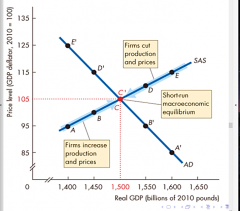
When the quantity of real GDP demanded = real GDP supplied. 𝐴𝐷 = 𝑆𝐴𝑆.

Equilibrium will remain at 𝐶𝐶′ in the short-run. Inventories (stocks of finished but unsold items) will increase if firms do not cut production and prices (when real GDP is greater than equilibrium GDP).

Firms produce quantities that maximise profits (on the 𝑆𝐴𝑆 curve), but equilibrium GDP can be above or below potential GDP, as the money wage rate is fixed (does not adjust to bring full employment) in the short run.

In the long run, money wage rate can adjust and real GDP moves towards potential GDP.

Front 22

Short-run equilibrium

Back 22

Front 23

Describe long run macroeconomic equilibrium

Back 23

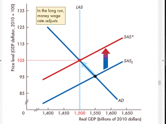
When real GDP = potential GDP.

When the economy is on the 𝐿𝐴𝑆 curve.

With excess labour demand, money wage rate rises. The short-run equilibrium is below potential GDP, and unemployment rate is above natural rate.

With excess labour supply, money wage rate falls. If the money wage rate is too low, short-run equilibrium is above potential GDP, and unemployment rate is below natural rate. Money wage rate adjusts in the long run, as wages are renegotiated in order to preserve their purchasing power. In both cases, the 𝑆𝐴𝑆 curve shifts so that the 𝑆𝐴𝑆 curve intersects 𝐴𝐷 at potential output. At 𝑆𝐴𝑆∗, the money wage rate has adjusted enough to bring full employment.

Front 24

Long-run Equilibrium

Back 24

Front 25

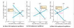
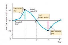
Describe the business cycle in the AS-AD model

Back 25

The graphs show different points of the business cycle.

Above full-employment equilibrium – An equilibrium in which real GDP exceeds potential GDP. Graph (a).

Output gap – The gap between real GDP and potential GDP.

Inflationary gap – The output gap when real GDP exceeds potential GDP.

Full-employment equilibrium – An equilibrium in which real GDP equals potential GDP. Graph (b).

Below full-employment equilibrium – An equilibrium in which potential GDP exceeds real GDP. Graph (c).

Recessionary gap – The output gap when potential GDP exceeds real GDP.

The economy moves from one type of macroeconomic equilibrium o another as a result of fluctuations in aggregate demand and in short-run aggregate supply.

The points 𝐴, 𝐵 and 𝐶 in graph (d) show the different equilibriums described in graph (a), (b) and (c) respectively.

Front 26

Business cycle in AS-AD model

Back 26

Front 27

Fluctuations in real GDP

Back 27