Ag Econ: Production-Single Input, Production Costs Supply And Price Determination, And Factor-Factor Sub And Prod-Prod Sub

Front 1

Production

Back 1

The process by which resources are transformed into products or services that are used in other production processes or consumed.

Front 2

What are three important questions to ask for production?

Back 2

What to produce? (product-product tradeoffs)

How much to produce? (input-product)

How to produce? (input-input substitution)

Front 3

What are important decisions to make for production?

Back 3

Resources are scarce and frequently costly

Competition forces efficiency and good planning

Profit is necessary for firm survival

Front 4

What are the production-physical relationships?

Back 4

Input-input

Product-product

Input-product

Front 5

How are outputs and inputs measured in Production-physical relationships?

Back 5

pounds, tons, bushels, kg., and acres

Front 6

What are the production-input classes?

Back 6

Land

Labor

Management (Entrepreneurship) - Decision making

Capital - every manufactured item that can be used in production

Front 7

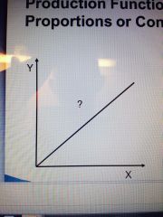
Fixed Proportions

Back 7

We increase all by the same percentage

Front 8

All ________ are increased in the same proportions.

Back 8

inputs

Front 9

Back 9

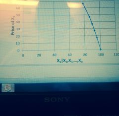
Total Physical Product (TPP)

Front 10

Y = _______ = f (X1 l X2, X3...., Xn)

Back 10

TPP

Front 11

TPP or Y ___________ at a(n) ______________ rate, then ______________ at a ______________ rate before it reaches its peak/maximum.

Back 11

increases

increasing

increases

decreasing

Front 12

Beyond the peak, TPP may begin to ________ even as X1 continues to _____________.

Back 12

decline

increase

Front 13

Define Marginal Physical Product (MPP)

Back 13

The amount added to TPP when another unit of input is used; the slope of the TPP curve

Front 14

Define the Average Physical Product

Back 14

TPP divided by the quantity of input

Front 15

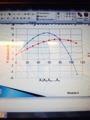
What is the blue line?

What is the red line?

Back 15

Blue line = MPP

Red line = APP

Front 16

Where is stage 1 located on an MPP and APP graph?

Back 16

Before MPP and APP cross

Front 17

Where is stage 2 located on an MPP and APP graph?

Back 17

From when the line of MPP and APP cross until the line of MPP hits zero

Front 18

Where is stage 3 located on an MPP and APP graph?

Back 18

Starting when the line of MPP hits zero

Front 19

Define Stage 1

Back 19

APP is increasing throughout, MPP is greater than APP, MPP increases then decreases; irrational

As long as the marginal contribution is greater than the average, add more input

Front 20

Define Stage 2

Back 20

APP is decreasing throughout, MPP is less than APP, MPP goes to zero; rational

Front 21

Define Stage 3

Back 21

MPP is negative; irrational

Front 22

When do you use more of the input?

Back 22

If the marginal benefit>marginal cost (in this case the input)

As you use more, the marginal benefit will decrease because MPP will decrease as you use more.

Front 23

When do you use less input?

Back 23

If the marginal benefit<marginal cost

As you use less, the marginal benefit will increase because MPP will increase as you use less.

Best decision: marginal benefit = marginal cost

Front 24

Define Total Value Product (TVP)

Back 24

TPP multiplied by the price of the product (output)

Front 25

Define Average Value Product (AVP)

Back 25

TVP divided by the number of units of the variable input

Front 26

Define Marginal Value Product (MVP)

Back 26

The change in TVP divided by the change in the variable input

Front 27

Define Total Factor Cost (TFC)

Back 27

the Variable Input multiplied by the price of the input (factor)

Front 28

Define Marginal Factor Cost (MFC)

Back 28

the change in TFC divided by change in the variable input

Front 29

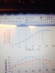
What does the blue line represent in the top graph?

Back 29

TVP

Front 30

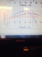
What does the blue line represent?

Red line?

Orange line?

Back 30

MVP

AVP

MFC

Front 31

What does this line represent?

Back 31

Input demand

Front 32

If we have improved technology and doubled the output for every input level, what will happen to the lines in the graphs?

Back 32

Shift upward

Front 33

Use marginal unit of the input until the _____________________ is equal to the Marginal Factor Cost.

Back 33

Marginal Value Product

MVP = MFC

Front 34

Aggregate supply

Back 34

Profitability

Number of firms

Risk and government policies

Front 35

Opportunity costs are _________ costs.

Opportunity costs are true ___________________.

Back 35

Implicit

costs of production

Front 36

Define Opportunity Cost

Back 36

the value of output that could have been obtained from an alternative use

Front 37

Define implicit cost

Back 37

opportunity cost that does not involve a money payment or market transaction

Ex: owned land, tractor that is owned

Front 38

Define explicit cost

Back 38

cost that involves a money payment and usually a market transaction. Also called out-of-pocket or accounting cost.

Front 39

Define Bookkeeping profit (accounting profit)

Back 39

occurs when all operating costs and overhead costs are exceeded by revenues so that a net balance remains

Front 40

Define economic profit

Back 40

occurs when revenues exceed the total of all explicit as well as implicit costs. Considers alternative uses of the resources or opportunity costs

Front 41

Define fixed costs

Back 41

costs that do not change as the quantity of output changes

Front 42

Define variable costs

Back 42

costs that change as the quantity of output changes

Front 43

In the immediate short run, meaning now, all _____________ are fixed.

Back 43

resources

Front 44

_________________ is a short run concept.

Back 44

Diminishing returns

Front 45

Ultimate long run: all _____________ are variable.

Back 45

Resources

Front 46

What is the total revenue equation?

Back 46

Price of output * Price of the input

Front 47

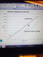
What is A?

B?

Back 47

A = Profit

B = Loss

Front 48

Define marginal cost

Back 48

the change in total cost divided by the change in output; the price of the input divided by the MPP

Front 49

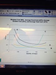
What does A represent?

B?

C?

D?

Back 49

A = ATC

B = AFC

C = MC

D = AVC

Front 50

Define marginal revenue

Back 50

the change in total revenue divided by the change in output

Front 51

What is the profit in the graph? (What area do you shade?)

Back 51

MC vertical to ATC then shade it all the way across

Front 52

What happens if price is below ATC?

Back 52

There is no economic profit.

Front 53

When will firms supply goods in the short run?

Back 53

If the price is greater than AVC.

The firm's short-run supply curve is Marginal Cost above Average Variable Cost

Front 54

Define Elasticity of supply

Back 54

Percentage change in quantity supplied divided by percentage change in price.

Generally positive

Supply can either be elastic (>1) or inelastic (<1)

Front 55

As length of run ___________, supply becomes more ________ because of the ability to change more of the resource base.

Back 55

increases

elastic

Front 56

Supply shifters (longer run)

Back 56

Technology

Price of the inputs

Number of firms in the industry

Change in the price of the output causes movement along the curve (does not shift the whole curve)

Front 57

Define surplus

Back 57

If the prices are above equilibrium, quantity supplied will be greater than quantity demanded

Front 58

Define shortage

Back 58

If the prices are below equilibrium, quantity demanded will be greater than quantity supplied

Front 59

Bumper crops do what?

Back 59

Shift supply to the right

Front 60

Crop failures do what?

Back 60

shift supply to the left

Front 61

What does factor-factor substitution look like?

Back 61

f (X1, X2 l X3, X4....., Xn)

Front 62

Isoproduct or Isoquant Curve

Back 62

Represent levels (amounts) of output, Yn.

Front 63

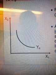
What curve is this?

Back 63

Isoproduct or Isoquant Curve

Front 64

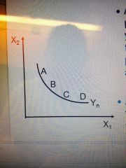
As you move from A to D, what happens?

Back 64

You substitute factor 1 for factor 2 while producing the same amount of output

Front 65

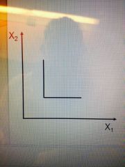
What does a right angle suggest?

Back 65

Isoquants at right angles suggest that fixed proportions or zero substitution of one input for the other

Factors 1 and 2 are one fixed combination of two inputs

Front 66

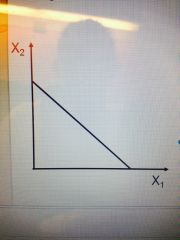
What does this straight line suggest?

Back 66

Isoquants in straight lines suggest perfect substitution of one factor for the other

Front 67

What is the negative of the slope of the isoquant called?

Back 67

Marginal rate of substitution (MRS) or the Marginal rate of technical substitution (MRTS)

^positive since the slope is negative

Front 68

Isocost lines

Back 68

Show the cost of various input combinations

On each line, the total cost is constant

The slope of the line shows how the market values one input versus the other

Front 69

Define Marginal Rate of Product Substitution

Back 69

amount of one product given up to produce another product

calculated as the slope of the production possibilities curve

Front 70

Define expansion path

Back 70

shows how output will change as resources change