585: Optimization Techniques In Systems Engineering

Front 1

Optimization Techniques

Back 1

A collection of techniques for determination of the best (optimal) course of action of a decision problem under the restriction of limited resources and other constraints

Front 2

Constrained vs unconstrained optimization

Back 2

unconstrained optimization has no constraint on the region of search

Front 3

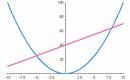
Unimodal vs bimodal functions

Back 3

Unimodal functions: have a single extreme value

Bimodal functions: have two extreme values

Front 4

Where to look for extreme values

Back 4

boundaryies of ourfunction

discontinuities in our function

Front 5

Concave

Back 5

ANY line connecting two points on the objective function surface lies entirely below the surface

Front 6

Convex

Back 6

ANY line connecting two points on the objective function surface lies entirely above the surface

Front 7

convex set

Back 7

any two points on the boundary of the search region can be connected by a straight line that lies ENTIRELY IN the region

Front 8

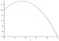
Unrestricted functions of a single variable

(problem)

Back 8

find minimum/maximum of y=f(x)

Front 9

Unrestricted functions:

Condition for extreme value

Back 9

if
f ' (x)=0

then x=a may be an extreme value

Front 10

Unrestricted functions:

How to determine if a possible extreme value is a maximum or minimum

Back 10

minimum:
f " (a) > 0

maximum:
f " (a) < 0

if f '' (a) = 0 and f ''' (a) = 0 then examine f '''' (a)

Front 11

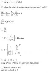
Unrestricted functions in multiple variables:

steps for solving

Back 11

1) ∆'y=0 --> ∂y/∂xi=0 for all i

(this gives us our possible extreme of x*=(x1*,x2*,...))

2) A= Hessian

3) A1=a11

A2= det(B2)

where B2=
[a11 a12
a21 a22]

A3=det[B3]

where B3=
[a11 a12 a13
a21 a22 a23
a31 a32 a33]

etc.

3) minimum: A1>0, A2>0, A3>0, ...
maximum: A1<0, A2>0, A3<0, ...

Front 12

Hessian

Back 12

A=
[a11 a21 a31
a12 a22 a32
a12 a23 a33]

where aij=d^2(y)/(dxi*dxj)

i=row
j=column

Front 13

Newton Raphson Method

Back 13

1) select x0

2) evaluate F^k and Jacobian, J^k, and solve

J^k*z=-F^k

for z

(z is defined as z=x^(k+1)-x^k)

3) if |z|<ε stop repeating

we use x^(k+1)

x^(k+1)=z+x^k

4) otherwise go to step 2)

Front 14

Jacobian Matrix

Back 14

J^k=
[df1/dx1 df1/dx2 ... df1/dxn
df2/dx1 df2/dx2 ... df2/dxn
.
.
.
dfm/dx1 dfm/dx2 ... dfm/dxn]

Front 15

Kuhn Tucker

Back 15

conditions that are necessary for a solution in NON-linear programming to be optimal

Front 16

Lagrange Multiplier

Back 16

a method for finding the maximum/minimum of a function subject to constraints

Front 17

Newton Raphson

Back 17

method for finding successively better approximations to the zeros (or roots) of a real-valued function

Front 18

Lagrange Multiplier

(step by step method)

Back 18

Front 19

Sufficient Conditions for Kuhn Tucker Method

Back 19

*Maximum (ie not a minimum):

Concave y
Constraints form a convex set

*Minimum (ie not a maximum):

Covex y
Constraints form a convex set

Front 20

Method of Slack Variables

(use)

Back 20

Used to change an inequality constraint into an equality constraint

Front 21

Method of Slack Variables

(step by step)

Back 21

(1) put constraint in gi<=0 form

(2) add a new x_(k+1)^2 variable and set =0 instead of <=0

gi+x_(k+1)^2=0

(3) these are your new constraints
proceed with previous methods