![]()
![]()
![]()
Use LEFT and RIGHT arrow keys to navigate between flashcards;
Use UP and DOWN arrow keys to flip the card;
H to show hint;
A reads text to speech;
146 Cards in this Set
- Front
- Back
|
Define Statistics |
The science that relates data to specific questions of interest. Methods to gather, summarize and display data and draw answers from data |
|
|
Two types of statistics |
Descriptive Inferential |
|
|
Why do we need statistics? |
Uncertainty in data Generalize beyond the sample |
|
|
Three primary sources of uncertainty in data collected in social sciences research |
Empiricism Testability Objectivity |
|
|
Data |
Numbers, the result of measurements |
|
|
Variable |
An event or behavior that can assume more than two values |
|
|
Constant |
A construct that has only one value |
|
|
Qualitative/categorical variable |
A variable that has discrete categories |
|
|
Quantitative/continuous variable |
A variable that has assigned numbers and the values are ordered in a meaningful way |
|
|
Population |
Individual/group that represents all members of group or category of interest Parameter |
|
|
Sample |
Subset that is used to represent a population Statistic |
|
|
Four scales of measurment |
How variable/numbers are defined and categorized Nominal Ordinal Interval Ratio |
|
|
Nominal scale |
Categories that are different from each other, but in kind, not degree |
|
|
Ordinal scale |
A scale of measurement that permits events to be rank ordered |
|
|
Interval scale |
A scale of measurement that permits rank ordering of events with the assumption of equal intervals between adjacent events |
|
|
Ratio scale |
A scale of measurement that permits rank ordering of events with the assumption of equal intervals between adjacent events and a true zero point |
|
|
Why are scales of measurement important |
Each scale has different properties that determine the appropriateness for use of certain statistical anlyes |
|
|
Descriptive statistics |
Used to describe characteristics of distribution of scores Makes a simplified record of something Makes it easy to get to main point Makes record systematic Basis for inferential statistics |
|
|
Types of descriptive statistics |
Measures of central tendency Dispersion/distribution/variability |
|
|
Measure of central tendency |
One score that summarizes the data The most representative score of a set of observations |
|
|
Measures of central tendency |
Mode Median Mean |
|
|
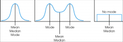
Measures of central tendency: symmetrical distributions |
|
|
|
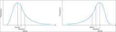
Measures of central tendency: skewed distributions |
|
|
|
Mode |
The score in a distribution that occurs most often |
|
|
Median |
The number that divides a distribution in half |
|
|
Mean |
The arithmetic average of a set of numbers. Adding all scores in a set and then dividing by number of scores |
|
|
Preferred measure of central tendency |
Mean because it best resists fluctuation between different samples and uses every value in data |
|
|
Three situations using measure of central tendency other than mean |
1. Use median when scores in a distribution are skewed (positive or negative) 2. Use median when there are a few extreme scores (high or low outliers) 3. Use mode for nominal data and median for ordinal data |
|
|
Frequency distribution table |
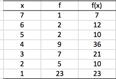
An organized tabulation of the number of individuals located in each category of a measurement scale |
|
|
Primary columns |
1. Identify highest and lowest scores. First column lists the categories that make up the scales of measurement (X) 2. Second column lists the frequency associated with each score (or categories of scores) (f) |
|
|
Four rules of making a grouped frequency distribution table |
1. Should have about 10 intervals 2. Width of each interval should be relatively simple 3. Bottom score should be multiple of width 4. All intervals should be same width |
|
|
Calculate N from a frequency table |
The sum of the frequency, f, column = number of scores/size of the sample |
|
|
Calculate sum of X from frequency table |
The sum of the frequency of x, f(x), column |
|
|
Calculate M from frequency table |
Sum of x/N Sum of f(x)/sum of f |
|
|
Variability |
The dispersion or spread of scores; a quantitative measure of the degree to which scores in a distribution are spread out or clustered together |
|
|
Variability - descriptive |
Measure degree to which scores are spread out/clustered together in distribution |
|
|
Variability - inferential statistics |
Provides measure of how accurately any individual score or sample represents entire pop |
|
|
Range |
Total distance covered by the distribution from the highest score to lowest score Xmax (highest score) - Xmin (lowest score) |
|
|
Range's primary limitation |
Very crude, only based on two scores in entire distribution |
|
|
Interquartile range |
The distance covered by the middle 50% of the distribution (Q1 and Q3) |
|
|
Standard deviation |
Average distance from each score to mean |
|
|
Abelson's Laws |
1. Chance is lumpy 2. Overconfidence abhors uncertainty 3. Never flout a convention just once 4. Don't talk Greek if you don't know the English translation 5. If you have nothing to say, don't say anything 6. There is no free hunch 7. You can't see the dust if you don't move the couch 8. Criticism is the mother of methodology |
|
|
Abelson Ch 1 Main Points |
Cannot make claim with stand-alone statistics Importance of comparison Standards of comparison (control groups) can reduce misleading statistical interpretations Several possible candidate explanations (chosen explanation becomes claim) Natural tendency for systematic conclusions over chance Null hypothesis testing Significance tests provide limited information Single studies are not definitive |
|
|
MAGIC criteria |
Magnitude, articulation, generality, interestingness, credibility |
|
|
Magnitude |
The strength of a statistical argument is enhanced in accord with the quantitative magnitude for its qualitative claim |
|
|
Articulation |
The degrees of comprehensible detail in which conclusions are phrased |
|
|
Generality |
The breadth of applicability of the conclusions |
|
|
Interestingness |
Must have potential, through empirical analysis, to change what people believe about an important issue |
|
|
Credibility |
The believability of a research claim, both methodological and theoretical coherence |
|
|
Style |
Dimension along which different possible presentations of same result can be arrayed Assertive/incautious style vs liberal style |
|
|
Convention |
Standards to be followed (e.g. significance level) |
|
|
Steps to calculate standard deviation |
(Sum of X - mean)/N |
|
|
Deviation scores |
Difference between each individual score in distribution and mean of distribution (X-mean) |
|
|
Square deviance scores |
Difference between individual scores and mean, squared (X-mean)^2 |
|
|
Sum of squared deviance scores (SS - sum of squares) |
Sum of all individual score and mean differences, squared Sum of (X-mean)^2 |
|
|
Variance |
SS/(N-1) or SS/df |
|
|
Square root of variances |
SD = square root of (SS/df) |
|
|
Three things that help researchers determine meaningfulness of data |
1. Statistical significance - confident results aren't due to chance 2. Practical significance - effect size, clinical significance 3. Confidence interval - precision of statistic, confidence statistic falls in certain range |
|
|
Three possibilities that can account for a distribution of scores (Abelson Ch 2) |
1. Variability of scores can be entirely explained by chance factors 2. Variability of scores can be enitrely explained by systematic facotrs 3. Variability of scores can be explained by both systematic and chance factors *1 & 2 are most parsimonious *Statistical significance 1 vs 2 0r 3 |
|
|
Three types of random influences or chance occurrences that might influence data |
1. Random generation 2. Random sampling 3. Random assignment |
|
|
Fundamental characteristics of normal distribution |
1. Symmetrical 2. Unimodal 3. Asymptotic |
|
|
Why is normal curve/distribution important? |
Links data to probabilities |
|
|
Central limit theorem |
Describes distribution of sample means using shape, central tendency, and distribution |
|
|
Central limit theorem: shape |
Normal approximation: the distribution of sample means will be almost perfectly normal if - population from which samples are selected is a normal distribution - the number of scores (n) in each sample is relatively large (30 +) |
|
|
Central limit theorem: central tenedency |
Mean of distribution of sample means (expected value of M) is always equal to population mean |
|
|
Central limit theorem: variability |
Standard error of M (σ subm) - standard deviation of sample means 1. provides measure of how difference is expected from one sample to another 2. describes how well individual sample mean represents entire distribution |
|
|
Size of standard error is function of two things: |
1. Size of sample 2. The population standard deviation (most of the time we do not need to have the population standard error, therefore we must estimate from sample data) |
|
|
Standard error |
The standard deviation of the frequency of distribution The measure of how much random variation we would expect from samples of equal size drawn from a population |
|
|
Test-statistic |
Standardized value calculated from sample data during hypothesis test Determine whether to accept or reject null hypothesis Compares data with what is expected under null hypothesis Observed effect or difference/SE of effect |
|
|
Two types of deviation from normality in distribution: |
Positive skew or negative skew |
|
|
Probability |
Likelihood of an event occurring |
|
|
Positive right skewed distribution |
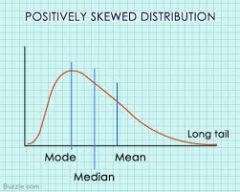
Tail goes to right, mean is right of peak, median, and mode |
|
|
Negative left skewed distribution |
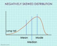
Tail goes to left, mean is left of peak, median, mode |
|
|
Standardization |
Process of converting raw score (difficult to interpret by themselves) to a standard score (metric or unit easily interpretable) T-score Z-score |
|
|
Z-score: how to interpret |
z = (raw score X -mean)/SD negative sign is below the mean, zero is the mean, and positive is above mean Number represents number of SDs Link up with different probabilities within SD High z-score = more extreme score |
|
|
Numerator test-statistic |
Observed effect (signal) |
|
|
Denominator test-statistic |
Standard error of effect, variation (noise) |
|
|
Goal of hypothesis testing |
Rule out chance (sampling error) as plausible explanation for results from a research study - statistical significance - always two explanations for pattern 1. systematic factors - meaningful 2. random influence - not meaningful |
|
|
Four steps of hypothesis testing |
1. State hypothesis and specify alpha level - reject/accept null 2. Locate critical region - center dist due to chance - tail not due to chance 3. Calculate test statistic - t, z, F, corr coefficient, test = effect/variation 4. Make a decision - data, test statistic, critical region, accept or reject null |
|
|
p value |
Probability null hypothesis is correct Probability of getting results you did given null is true Probability of obtaining statistic of given size from a sample of a given size by chance (random error) |
|
|
alpha |
Level of significance Probability value used to define very unlikely sample outcomes if null is true The a priori probability of falsely rejecting null that research is willing to accept |
|
|
General Linear Model |
A common mathematical foundation of several different stat models ANOVA, ANCOVA, MANOVA, MANCOVA, ordinary linear regression, t-test, f-test |
|
|
GLM equation |
Yi = B0 + B1X1i + εi Yi = value of DV or outcome, expected value B0 = intercept term, constant effects, value of Yi when all X's are 0 B1 = regression coefficient for variable X, how much does X influence Y (slope) X1i = score of x for person or case 1 εi = residual error, how far is person's actual score from expected score |
|
|
GLM graphically depicted |
In notes Slope of best fit line, how far data falls from expected |
|
|
T-test |
Compare two means to see if significantly different from one another |
|
|
Three types of t-tests |
1. One- sample 2. Paired-samples 3. Independent-samples |
|
|
One-sample |
Data collected from one sample under one condition at one time Does sample mean differ from pop mean or meaningful number? |
|
|
Paired-samples |
Observations that are not totally dependent 1. Within-subjects design (same people under certain conditions) - DV or outcome variable is assessed at multiple occasions for each participant 2. Matched data (e.g. parent/children) |
|
|
Independent samples |
Comparing two totally separate samples (no overlap) Compare groups - randomized control trial comparing random vs control Between-subjects experimental design Quasi-independent variable (gender) |
|
|
Assumptions of t-tests |
Compare two means |
|
|
Limitations of t-tests |
Can only compare two means (only one IV with two conditions), limited to one IV Limited to one IV with two conditions (can only compare two means) |
|
|
Type I error |
False positive (say difference but not) When null hypothesis is true but it is rejected alpha = chance of making type I error Conclude difference/effect but it isn't (more concerned with type I error) |
|
|
Type II error |
False negative Null hyp is false but is accepted as true β (power) = chance of making Type II error Conclude no effect, but there is |
|
|
Why use ANOVA based on Type I/II errors |
ANOVA tests the difference among all groups simultaneously, avoiding inflation of experimentwise alpha Conducting several separate t-tests instead of one overall ANOVA increases experimentwise alpha level, increasing type I erro |
|
|
Testwise alpha |
Alpha level for each individual hypothesis test Acceptable amount of tolerance for Type I error for one test |
|
|
Experimentwise alpha |
Total probability of type I error accumulated from all separate tests of experiment r |
|
|
one-way ANOVA |
When you want to compare two or more means (three) One IV (factor) with two or more conditions (levels) |
|
|
General logic of ANOVA |
Decompose variance to test mean differences by analyzing variance Decompose total variance/variability into smaller parts Total variance --> between treatments *measure difference due to 1. systematic treatment effects 2. random unsystematic factors* Total variance --> within treatments *measure difference due to 1. random unsystematic factors* |
|
|
Factor |
Independent variable or quasi independent variable that designates groups being compared |
|
|
Levels |
Conditions of the independent variable or value that make up factor (e.g. quasi IV - gender; IV - neutral, happy, sad) |
|
|
k |
Number of conditions/levels for factor |
|
|
n |
number of scores in each treatment/condition |
|
|
N |
Total number of scores in entire study |
|
|
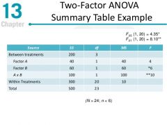
SS |
Sum of squares, sum of squared deviations, sum of squared differences from the mean Sum of (x - mean)^2 |
|
|
MS |
Mean square - estimate of variance across groups SS/df |
|
|
df |
Degrees of freedom, how many scores are free to vary within sample |
|
|
F |
test statistic for ANOVA, uses variance variability as measure of diff between group because there is more than one group MSbetween/MSwithin |
|
|
F numerator |
Variance between treatments (effect) |
|
|
F denominator |
Error term, random unsystematic variability (noise) |
|
|
Factorial design |
Two or more IV When study involves more than one factor or IV - completely crossed (each level with each IV appears in combo with every other level of IV |
|
|
dfTotal |
N-1 dfw +dfb |
|
|
dfWithin |
Sum of (n-1) = sum of df N - k |
|
|
dfBetween |
k - 1 |
|
|
Main effects |
Average effect of A when you average across B |
|
|
Controlled or partial effects |
Main effect of factor A in factorial design is different than in one-way ANOVA because controlling for effect |
|
|
Interactions |
The joint synergistic effect of A and B on DV The relationship between factor A and te DV difference across different levels of factor B Occurs when the effect of on IV on DV varies across different levels of another IV |
|
|
dfTotal |
N-1 |
|
|
dfBetween |
# of cells - 1 k - 1 |
|
|
dfWithin |
N - # of cells N - k |
|
|
dfA |
kA - 1 |
|
|
dfB |
kB - 1 |
|
|
dfAxB |
dfBetween - dfA - dfB |
|
|
ANOVA table |
|
|
|
Difference between descriptive statistics reported at top of factorial ANOVA and estimated marginal means |
Estimated marginal means - means when controlling for all other variables Descriptive statistics - raw means |
|
|
Two general types of effect size estimates |
Mean differences Associations |
|
|
Cohen's d |
effect size indicator General form: M1 - M2/SD Express mean diff in SD units |
|
|
Variations on d |
Same general form, but diff SD used Cohen's d = M1 - M2/SDpooled (mot appropriate when variances/sample size are equal) Glass's delta = M1 - M2/SD control (when N is diff/diff homogeneity in variance) Hedge's g = M1 - M2/SD*pooled (deals with bias due to sample size) |
|
|
Guidelines for Cohen's d |
small = .20 medium = .50 large = .80 |
|
|
Effect size indicator for ANOVA |
Omega squared ω², eta squared η² small = .01 medium = .06 large = .141 |
|
|
Point estimate |
Use single estimate of unknown quantity (e.g. mean) High precision, low confidence |
|
|
Interval estimate |
Use range of values as estimate of unknown quality Low precision, high confidence |
|
|
Precision vs confidence: tradeoff |
Point estimates are very precise - specify one value, but can't be confident correct Interval estimates are less precise - specify range of values, but can be confident estimate of pop parameter is in interval |
|
|
95% confidence interval for mean |
CI95 = M +/- (t95)(Sm) |
|
|
95% confidence interval for any estimate |
CI95 = Estimate +/- (t95)(EstimateSb) |
|
|
3 characteristics of relationship between two variables described by correlation coefficent |
1. Direction - indicated by sign of correlation (positive = same direction, negative = different direction) 2. Form 3. Strength |
|
|
Factors influencing strength of correlation |
1. Restricted range of scores represented in data - need people to represent all ranges of both scales 2. Outliers - one or two very extreme data points can have dramatic impact (more impact on small sample size than large sample size) |
|
|
r |
Provides an estimate of the degree of relationship between two variables (regression coefficient) |
|
|
r² |
Preferred way to describe relationship between two variables (coefficient of determination) Interpretation more straightforward, shows how much overlap in variance of two variable Shows how much percentage of Y is captured by X How much variance in outcome variable is accounted for by variance in predictor variable in regression |
|
|
Four types of correlation coefficients |
Pearson's correlation Spearman correlation Point-biserial correlation Phi coefficient |
|
|
Pearson's correlation coefficient |
Linear, variables interval/ratio continuou |
|
|
Spearman |
Nonlinear, ordinal |
|
|
Point-biserial |
One dichotomous variable and one continuous varibale, very similar to independent samples t-test |
|
|
Phi |
Two dichotomous variables (connected to Chi squared) Can do categorical variables with more than two categories |
|
|
Covariance and correlation |
Association between two variables, strength |
|
|
Covariance |
Not directly interpretable - on scale of two variables (unstandardized coefficient) Compare covariance of two data sets on same metric, can get sense of relationship |
|
|
Correlation |
Standardized coefficient Cross products: positive correlation |