Reading...
![]()
Play button
![]()
Play button
![]()
Use LEFT and RIGHT arrow keys to navigate between flashcards;
Use UP and DOWN arrow keys to flip the card;
H to show hint;
A reads text to speech;
32 Cards in this Set
- Front
- Back
|
Decision tree
|
-Direct access Model
-Branch point for each letter -It takes a certain amount of time to get from one level to another -The tree is constructed so that the constraints of English orthography are preserved. -Not every combination of letters is represented. -The essence of the model is that a serial search is involved. -Nonwords= exhaustive search -Words= terminating search |
|
|
Process
|
Trace the path of a given word for A T I S H N E T in sequence and take the address specified at the terminal node. Could discover no information in the lexicon at this address and conclude A T I S H N E T is not a word.
|
|
|
Predictions
|
-LDT: words < nonwords
-LDT: word length effect Shorter words < longer words |
|
|
Problems
|
-Empirical results = word length has no effect (null)
-It does not account for frequency -Doesn't specify if alphabetical/ arbitrarily |
|
|
Assumptions
|
Not conscious of going through each word but set dome type of deadline→ assumption that a branch won’t exist. All the entries on a page will be searched before a “no” decision is made. There is no branch or address if it is not a word and won’t exist in the lexicon.
|
|
|
Draw Diagram
|
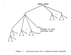
Decision Tree for Direct Access Lexcion
|
|
|
Serial Search Model
|
-Search Model
-Not direct access -Three access files = different input methods. Points to one entry in “master file” (lexicon). Entries are ordered by KF printed frequency -Tested on two tasks: LDT & ADT |
|
|
Predictions
|
-LDT: ambiguous = unambiguous
-ADT: ambiguous < unambiguous -Unambiguous must go thru exhaustive search -Equiprobable < unequiprobable homograph |
|
|
Findings & Problems
|
Findings:
LDT: ambiguous < unambiguous ADT: ambiguous < unambiguous Problems: -Why are ambiguous words slightly faster on the LDT? -Equiprobable = unequiprobable homographs -How to explain this? -How does the list get into our heads? |
|
|
Process
|
Frequency ordered list, go through entire list to see if a word exist in the lexicon: yes or no. High Frequency vs. Low Frequency= make prediction based on 1st encounter especially for an ambiguous word b/c only care if it exist somewhere on the list. Search further to find 2nd meaning. Same organization of words/ structure for ambiguous and non-words. What changes is the nature of the search. *Finding a way to access the master file, only stored once. Master File: has complete info about a word through hearing/ listening, pronouncing, spelling a word. **Reject Null also rejects model that made that prediction, when encounter a word, goes to the top of the list.
|
|
|
Draw Diagram
|
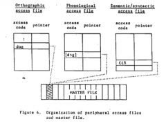
Master File
|
|
|
II. Word-recognition models
2. Interactive activation model (McClelland & Rumelhart) Purpose |
Perception results from excitatory and inhibitory interactions of detectors for visual features, letters, and words. Figure 1: Perceptual Processing is assumed to occur in a set of interacting levels, each communicating with several others where activation at one level spreads to neighboring levels. Excitatory messages increase the activation level of their recipients. Inhibitory messages de- crease the activation level of their recipients.
|
|
|
Interactive Activation Model
|
-Direct Access
-Computational Model -Reflects neurology -Connections: excitatory or inhibitory -Lateral inhibition within word level & letter level -Localist representation -One word, one node |
|
|
II. Word-recognition models
2. Interactive activation model (McClelland & Rumelhart) Assumptions: General |
1st we assume that perceptual processing takes place within a system in which there are several levels of processing. For visual word perception, we assume that there is a visual feature level, a letter level, and a word level, as well as higher levels of processing that provide "top-down" input to the word level. 2nd we assume that visual perception involves parallel processing. We assume that top-down processing works simultaneously and in conjunction with bottom-up processing that determine what we perceive.
|
|
|
IV. Ambiguity
2. IA model - multiple word nodes with either inhibitory or excitatory connections. Purpose |
Word Superiority Effect. 3 different input methods are taken into account (visual, acoustic, and higher level input. Only built to measure 4-letter words, see all letters at the same time, not limited to one letter we see.
|
|
|
IV. Ambiguity
2. IA model - multiple word nodes with either inhibitory or excitatory connections. Assumptions |
1. Several levels of processing
2. Spatial Parallel Processing & Parallel Processing (what words start with first letter “w” and does for each letter “work” across different levels: feature, letter, and word at the same time) 3. Top-own & Bottom-Up Processing (contextual evidence ex: wor ‘k’ get letter ‘d’ 4. Method of Interaction= Excitatory/ Inhibitory (like neurons from one node to another). |
|
|
IV. Ambiguity
2. IA model - multiple word nodes with either inhibitory or excitatory connections. Features |
I. Node (circles) for letters, words, features all unique (one node represents one entry) → have to connect to each other.
II. Connections= Excitatory/ Inhibitory could be nodes at same level , only between adjacent levels (across, up/down) have to go to next level first before go to one above it. III. Between adjacent levels only within levels. IV. Feature nodes are binary. Q: Is it Present/ Absent or not? PIC Ex: N and Activate feature→ any letter that has this feature ‘l’ letter matches most features will have the highest match (M L)….. Lateral Inhibition. |
|
|
IV. Ambiguity
C. Extensions of word recognition models 1. Serial search model (Consecutive entries (multiple pointers) vs. Non-consecutive entries) Assumptions |
1st Finding: Nonwords require an exhaustive search of the subset of the lexicon in order to determine that no entry is present which must take longer than a self-terminating search for a word. 2nd Finding: assumption that the most frequently accessed words near the beginning of the list of entries to be searched.
|
|
|
IV. Ambiguity
A. Relative frequency of senses (Equi-probable vs. Unequi-probable/polarized) 4 Types of Stimuli: (Ambiguity Decision Task: Exhaustive Search. Entire list) |
1. Equi-proable Homograph= equally frequent of occurring, related to each other. (ex: yard, patient)
2. Unequi-proable Homograph= one more frequently occurring than other. (ex: sentence less frequently occurring grammar vs. court, sound). 3. Ambiguous words= one meaning 4. Nonwords= legal spelling but not a word in English (ex: pote, glany) |
|
|
IV. Ambiguity
A. Relative frequency of senses (Equi-probable vs. Unequi-probable/polarized) Predictions |
Unambiguous words > homographs (according to time) & Equi-proable Homograph < Unequi-proable Homograph.
1. Unambiguous words take longer than homographs in the ambiguity decision task but not in the lexical decision task. → assumption that ambiguous words require an exhaustive search of the subset in the ambiguity decision task where homographs don’t. In lexical decision task, the search terminates for both types of words when the first meaning is accessed 2. The frequency effect for unambiguous words is much greater for lexical decisions than for ambiguity decisions→ supports that an exhaustive search is necessary for unambiguous words in ambiguity decision but not for lexical decision 3. Legal nonwords take longer than unambiguous words for lexical decisions 4. Ambiguity Decisions are much slower than Lexical Decisions. Lexical Decision Task: difference between a Terminating & Exhaustive Search VS. Ambiguity Decision Task: difference disappears and an exhaustive search is involved in both cases. |
|
|
IV. Ambiguity
A. Relative frequency of senses (Equi-probable vs. Unequi-probable/polarized) Found |
No significant Difference (Unambiguous words > homographs) & Unequi-proable > Equi-proable. In lexical decision task, Equiprobable Homographs NOT faster than Unamb Words.
|
|
|
B. Tasks (lexical decision & ambiguity detection).
Lexicon Task: Interruption |
find first entry is based on frequency, the 2 homographs not access at the same time, there’s an Interruption: takes time before stop process, restart it again (see if a word is ambiguous/ not).
|
|
|
B. Tasks (lexical decision & ambiguity detection).
Lexical Decision Task: defn & predictions |
Lexical Decision Task: dependent variable= decision time
Predictions: Ho: LDT unambig = LDT ambig H1: LDT unambig < LDT ambig H2: ALDT unambig >LDT ambig |
|
|
B. Tasks (lexical decision & ambiguity detection).
Ambiguity Detection Task: defn & predictions |
Based on own model, create hypothesis. Comparing ambiguous vs. unambiguous, choice of independent and dependent variables.
Predictions: Ho: ADT unambig = ADT ambig H1: ADT unambig < ADT ambig nonadjacent H2: ADT unambig > ADT ambig adjacent |
|
|
B. Tasks (lexical decision & ambiguity detection).
Ambiguity Decision Task: Definition |
Based on the search model, the method of reaching a decision would be to initiate a search, counting the number of lexical entries. “Yes” Response is executed= Self- Terminating vs. Exhaustive Search. For both Unambiguous Words & Nonwords an exhaustive search will be required.
|
|
|
B. Tasks (lexical decision & ambiguity detection).
Ambiguity Decision Task: Prediction |
1. There is no reason to expect unambiguous words to be classified any faster than nonwords. Unambiguous words may well take longer than nonwords.
2. There is no longer any basis for expecting high frequency unambiguous words, since in both cases the search does not terminate when the first entry is located. 3. Since a terminating search will be involved for ambiguous words, decision times should be fastest in this condition (Forster & Bednall: Notes3) |
|
|
Distributed Model
|
This model uses a ‘distributed representation’ in which a word is represented by a pattern of features analogous to a barcode. This model is also different in that it ‘learns’ a vocabulary by modifying the strength of the connections between processing units.Each entry is represented by activation in 216 Binary Features (have set of nodes with different levels of activation that represent a word). All 216 elements participate in the representation of every word.
|
|
|
Two Sets of 216 Binary Elements (DM)
|
1. Auto-Assoicate Network: allows you to access pronounications part of speech and meaning given the spelling.
2. Buffer Elements= Memory Buffer holds most recently accessed word (once access info, like reaching 2nd level). |
|
|
Learning (DM)
|
By changing strength of the connection between elements (Inhibitory/ Excitatory and get learning). Perfecting, teaching itself the pattern, meant to disambiguate ambiguous words.
|
|
|
Disambiguating Ambiguous Words (DM)
|
The sound of letter, which one (wine/ wind) maxiamal/ minimal activation= saturated.
ex: W I N D nodes for * activate first PIC * * * |
|
|
Energy Landscape (DM)
|
2 sense of ambiguousword= minima. For whole word, not just letter “I”and if word bias toward one way and rigid closer PIC. The steeper the slope, rigid move toward side that is more frequent. Rigid consequence of learning. Different patterns have different landscapes. The higher you go the more energy it has. Look to see how similar and close to the points/ pattern.
|
|
|
Energy (DM)
|
A number corresponding to the degree by which a "tote"~ (a pattern of activation) is consistent with the connection _____.
|