![]()
![]()
![]()
Use LEFT and RIGHT arrow keys to navigate between flashcards;
Use UP and DOWN arrow keys to flip the card;
H to show hint;
A reads text to speech;
6 Cards in this Set
- Front
- Back
|
VLOOKUP |
=VLOOKUP ( cellx, RangeName, ColumnNumber, 0 is exact match and 1 is for approximate match)
-exact = 0 -approximate = 1: the data needs to in ascending order
|
|
|
NESTED VLOOKUP
- a Vlookup within Vlookup |
Using a Vlookup to obtain Data1 from Range1, and then using that Data1 to extract Data2 from Range2
Get data from Range 1
=VLOOKUP(cell1,Range1,Column2,0)
We now use this data to obtain Data2 from Range2
=VLOOKUP ( VLOOKUP(cell1,Range1,2,0), Range2, column3,0)
|
|
|
CHOOSE |
=CHOOSE (Cell1 , value1,value2,value3,...,valuex) eg if cell1 = 3, then =CHOOSE = value3
Based on a number extracted from a function or cell1, you can select how to label it - numerically or with a "text" -You create characters for each value
eg use month funtion to extract a number =MONTH(Cell1)=3
=CHOOSE (MONTH(Cell1) ,jan ,feb, mar, apr,...,dec)
=mar
|
|
|
MATCH |
-If the information exist within a specified range, match will tell you the row number
Can be used nested in IFERROR formula, eg if not found then "n/a"
eg Cell7 code RTD23GET480
*NOTE To find the smallest value - the lookup area must be in descending order To find largest value - ascending order
=MATCH (Cell7, Column1, 0) = 8
this means that the datA in Cell7 is in 8th row
|
|
INDEX
|
Allows us to pull information out of a table given a Row and Column referance
= INDEX (highlight the contents of table only, Select Row, Select Column )
Give the table contents a range name eg Cost
=INDEX(Cost,Row,Column)
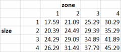
eg cell1 Size cell2 Zone 4 3 =index(cost,cell1,cell2)
|
|
|
INDEX & MATCH
note - you can create Data Validation for referance of Cell1 and Cell2 |
Use MATCH to find the location of Row and Column in table range and then to draw out the relevant data
= INDEX ( range , MATCH (cell1,highlightRow,0) MATCH (cell2,highlightColum,0) )
In MATCH you highlight the columns or rows you are searching data referanced in cellx |