Consumer Choices, Supply & Demand

Front 1

budget line/constraint

Back 1

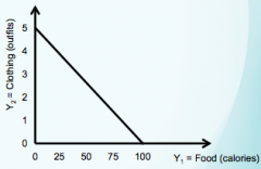
all possible combinations of 2 goods that may be purchased with entire budget

M ≥ Px*X + Py*Y

opportunity set is area under line, all consumption possibilities w/in budget limits

Front 2

cardinal vs ordinal utility

Back 2

cardinal is hypothetical numerical values (utils)

ordinal is based on ranking goods in order of preference

Front 3

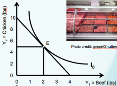
indifference curve

Back 3

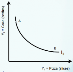
curve of all combinations of 2 good consumptions with same utility/satisfaction level

1. downward slope

2. complete

3. can't intersect

4. convex to origin

Front 4

MU

Back 4

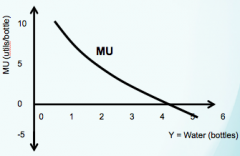
marginal utility

change in level of utility with consumption of one additional unit of a good

∆TU/∆Y

Front 5

TU

Back 5

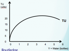
total satisfaction from consuming certain goods and services

Front 6

consumer behavior (assumptions)

Back 6

1. complete preference (always 1 good over the other)

2. consistent preference (always prefer the same thing over another thing)

3. nonsatiation (always want to consume more)

Front 7

law of diminishing marginal utility

Back 7

MU declines as more of a good or service is consumed in given time period (as increasingly more satisfaction is reached)

typically decreases the most after the first unit consumed

Front 8

complements

Back 8

goods that are either consumed or produced together

Front 9

perfect complements

Back 9

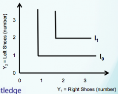
goods that must be consumed in a fixed ratio

Front 10

substitutes

Back 10

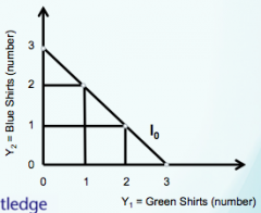
goods consumed either/or

compete for same resources in production

Front 11

MRS

Back 11

marginal rate of substitution

rate of exchange of one good for another leaving utility unchanged

∆Y2/∆Y1

Front 12

consumer equilibrium

Back 12

where slope of indifference curve = slope of budget line

MRS = price ratio

∆Y2/∆Y1 = -P1/P2

-MU1/P1 = MU2/P2

Front 13

elasticity

Back 13

% change in one economic variable with respect to the % change in another economic variable

Front 14

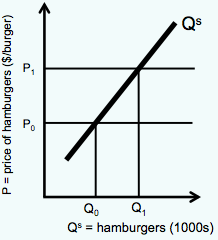
elasticity of supply

inelastic supply curve

elastic supply curve

unitary elastic supply curve

Back 14

%∆Qs / %∆P

unitless, becomes more elastic as time passes

unresponsive to changes in price (Es < 1)

responsive to changes in price (Es > 1)

change in price means equal change in quantity supplied (Es = 1)

Front 15

own-price elasticity of supply

Back 15

∆Qs in response to ∆P of that good

Front 16

cross-price elasticity of supply

Back 16

∆Qs in response to ∆P of a related good

Front 17

change in supply

Back 17

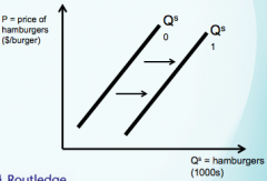
∆Qs due to change in another economic variable other than price of that good

shift of the entire supply curve

Front 18

change in quantity supplied (Qs)

Back 18

when ∆Qs is in response to ∆P of the good

movement along a supply curve

Front 19

demand curve

Back 19

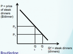
all possible combinations of prices and quantities consumed for a good, ceteris paribus''

market demand curve - sum of all horizontally

Front 20

Law of Supply

vs.

Law of Demand

Back 20

Q goods offered varies directly with P good

Q good demanded varies inversely with P good

Front 21

price elasticity of demand

inelastic demand curve

elastic demand curve

unitary elastic demand curve

Back 21

%∆Qd / %∆P

1% change P means relatively smaller %change Qd (|Ed| < 1)

relatively larger % change Qd (|Ed| > 1)

(|Ed| = 1)

Front 22

own-price elasticity of demand

Back 22

change in Qd in response to changes in P of same good

Front 23

cross-price elasticity of demand

Back 23

change in Qd in response to changes in P of a related good

Front 24

change in quantity demanded

Back 24

result of change in price of a good

movement along the demand curve

Front 25

change in demand

Back 25

change in economic variable other than P good

shift in the entire demand curve

Front 26

Engel's Law

Back 26

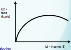
as income increases, proportion of income (M) spent on food declines

Front 27

income elasticity of demand (Em)

Back 27

%∆Qd / %∆M

change in demand from change in income

Front 28

normal good

inferior good

luxury good

necessity good

Back 28

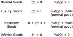
consumption increases with income rise (Em > 0)

consumption declines with income rise (Em < 0)

C increases at increasing rate with M (Em > 1)

C increases at decreasing rate with m (0

Front 29

supply

Back 29

relationship between price of a good and quantity available

determinants: 1. input prices, 2. technology, 3. prices of related goods, 4. number of sellers

Front 30

supply curve for individual firm

Back 30

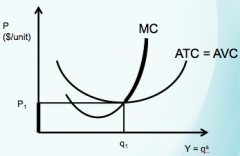
MC above the AVC curve

Front 31

determinants of demand

Back 31

own price

P related goods

M (Income)

tastes and preferences

expected prices

population

Front 32

shift in supply

Back 32

change in supply (movement whole supply curve)

change in quantity demanded (movement along demand curve)