Reading...
![]()
Play button
![]()
Play button
![]()
Use LEFT and RIGHT arrow keys to navigate between flashcards;
Use UP and DOWN arrow keys to flip the card;
H to show hint;
A reads text to speech;
105 Cards in this Set
- Front
- Back
|
Questions to ask yourself about a study.
|
How generalizabl are the findings?
What degree of clinical severity are being looked at? How matched are the cases and controls? how are the scores distributed in the study population? |
|
|
How do you look at the data in a study?
|
Determine what the saa looks like.
What trends are shown? What are the outliers (mathematicaly unusual scores)? What statistical tests are most appropriate? What is the typical value, central tendancy, or average response? How much spread, or variability, is there in the values? Highly variable = difficult to predict. Less variable = more predictable responses |
|
|
What are the main ways to display one variable, frequency distribution data?
|
Categorical Data:
*Bar chart *Pie chart Continuous Data: *Histogram *Dot plot *Box plot *Stem-and-leaf plot |
|
|
What are the main ways to display two variable, relationship data?
|
Categorical Data - Segmented bar chart
Continuous Data - Scatter plot |
|
|
What are the possible shapes of frequency distribution?
|
Modality - how many peaks does the curve have? unimodal = 1, bimodal = 2, multi-modal = >2
Is the curve semetrical or skewed? The tail end points in the direction of the skew. |
|
|
Arithmetric mean (average)
|
The sum of the values divided by the number of values.
|
|
|
Median
|
middle value, 50th percentile
|
|
|
Mode
|
the most common value
|
|
|
Geometric mean
|
antilog of the mean of the log data (for skewed data)
|
|
|
Weighted mean
|
when certain values carry ‘more weight’ or importance than others
|
|
|
If the mean = the median
|
the distribution is symmetrical
|
|
|
If the mean does not equal the median
|
the distribution is not symmetrical
|
|
|
What are the measures of central tendancy?
|
Mean
Median Mode Geometric mean Weighted mean |
|
|
What are the advantages of using the mean as a measure of central tendancy?
|
Uses all data
Algebraically defined |
|
|
What are the advantages of using the median as a measure of central tendancy?
|
Not distorted by outliers
Not distorted if skewed |
|
|
What are the advantages of using the mode as a measure of central tendancy?
|
Easy if categorical data
|
|
|
What are the advantages of using the Geometric Mean
as a measure of central tendancy? |
Transformed, same pros as mean
Good for skewed data |
|
|
What are the advantages of using the Weighted Mean
as a measure of central tendancy? |
Same pros as mean
Relative importance Algebraically defined |
|
|
What are the disadvantages of using the mean as a measure of central tendancy?
|
Distorted by outliers
Distorted if skewed |
|
|
What are the disadvantages of using the median as a measure of central tendancy?
|
Ignores most data
Not algebraic |
|
|
What are the disadvantages of using the mode as a measure of central tendancy?
|
Ignores most data
Not algebraic |
|
|
What are the disadvantages of using the geometric mean as a measure of central tendancy?
|
Only good if log transformation yields symmetrical distribution
|
|
|
What are the disadvantages of using the weighted mean as a measure of central tendancy?
|
Need good estimates of weights
|
|
|
Measures of variability
|
Range (minimum - maximum)
Percentiles – value of x that has n% of the observations below it is the nth percentile interquartile range = range between the 25th and the 75th percentiles or the central 50% Variance – average deviation from the mean s2 = Σ(xi – x)2/n - 1 Standard Deviation – square root of the variance s = sd = √ Σ(xi – x)2/n - 1 |
|
|
What are the advantages of using range to determine variability?
|
Easy to determine
|
|
|
What are the disadvantages of using range to determine variability?
|
Uses only 2 data pts.
Distorted by outliers Increases with sample size |
|
|
What are the advantages of using Inter-Quartile Range
to determine variability? |
Unaffected by outliers
Independent of sample size Good for skewed data |
|
|
What are the advantages of using Variance to determine variability?
|
Clumsy to calculate
Uses every data pt. Algebraic |
|
|
What are the advantages of using Standard Deviation
to determine variability? |
Same as variance
Units of measure = units of raw data Easy to interpret |
|
|
What are the disadvantages of using Inter-Quartile Range
to determine variability? |
Clumsy to calculate
Not good for small samples Uses only 2 data pts. Not algebraic |
|
|
What are the disadvantages of using Variance to determine variability?
|
Units of measure = square of the raw data units
Sensitive to outliers Not good for skewed data |
|
|
What are the disadvantages of using Standard Deviation
to determine variability? |
Sensitive to outliers
Not good for skewed data |
|
|
Don't forget to look at your slide for the stem and leaf plot
|
Sept 18th Lecture
|
|
|
Don't forget to look at your slide for the Box and whiskers plot
|
Sept 18th Lecture
|
|
|
Why do we care about central tendency and variation?
|
* Answers what is the typical value - is it what we expect, how does it compare to other groups?
* Will help us understand how confident we are in our point estimate * Provides guidance for what statistical test is most appropriate |
|
|
Refer to Mossad article on Zinc Losenges Table 1
How generalizable are the findings for a 70 year old Asian female patient? |
These findings are not generalizable to a 70 year old Asian woman.
|
|
|
Refer to Weaver article on Sleep Apnea Table 2
What is the degree of clinical severity in the patients in this study? |
Comparing the normal range to the range of scores exhibited by the study participants, there is a large variance in the degree of severity.
|
|
|
Refer to Valuck article on B12 deficiency Table
How matched are the case and controls? Difference in history of acid suppression therapy usage? |
There is a good match between the percentages of male/female, age, and therapy.
|
|
|
Refer to Perez article on Antidepressants Table 1
How is the HAMD, a measure of depression severity, distributed in the study population? |
The curve is skewed to the left.
|
|
|
What are the four main ways to measure risk?
|
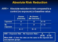
* Absolute Risk Reduction (ARR)
* Number Needed to Treat (NNT) * Relative Risk (RR) * Odds Ratio (OR) |
|
|
Calculating Absolute Risk Reduction
|
|
|
|
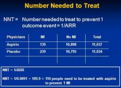
Calculate Number Needed to Treat
|
|
|
|
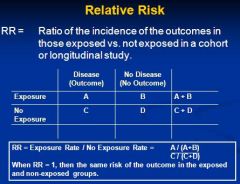
Calculate Relative Risk
|
|
|
|
Calculate Relative Risk
|

|
|
|
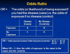
Calculate Odds Ratio
|
|
|
|
Bias
|
A systematic difference between the results obtained by a study and the true state of affairs
|
|
|
Blinding (definition, single, double)
|
When the patients, clinicians, and assessors of response to treatment are unaware of of the treatment allocation (double-blind), or when the patient is aware of the treatment received but the assessor of the response is not (single-blind). Also called masking.
|
|
|
Blocking
|
Also called stratification. Grouping experimental units that share similar characteristics into a homogenous block or stratum.
|
|
|
Cohort
|
A group of individuals, all without the outcome of interest (e.g. disease), is followed (usually prospectively) to study the effect on future outcomes of exposure to a risk factor.
|
|
|
Controls (control group)
|
A term used in comparative studies, e.g. clinical trials, to denote a comparaison group. This group of individuals either does not have the disease or is not receiving the treatment.
|
|
|
Experimental study
|
The investigator intervenes in some way to affect the outcome
|
|
|
Geometric mean
|
A measure of location for data whose distribution is skewed to the right; it is the antilog of the arithmetic mean of the log data
|
|
|
Incidence
|
The number of new cases of a disease in a defined period of time divided by the number of individuals suceptible at the start or mid-period of the period
|
|
|
Inclusion/Exclusion criteria
|
A definition of which patients are to be recruited
|
|
|
Intention-to-treat
|
All patients in the clinical trial are analysed in the groups to which they were originally assigned
|
|
|
Interquartile Range (IQR)
|
The difference between the 25th and the 75th percentiles; it contains the central 50% of the ordered observations
|
|
|
Longitudinal study
|
Follows individuals over a period of time
|
|
|
Matching
|
A process of creating (usually) pairs of individuals who are similar in respect to variables that may influence the response of interest
|
|
|
Mean
|
A measure of location obtained by dividing the sum of the observations
|
|
|
Measures of Risk
|
EER, CER, RR, OR, ARR, RRR, and NNT
|
|
|
Median
|
A measure of location that is the middle value of the ordered observations
|
|
|
Mode
|
The value of a single variable that occurs mist frequently in a data set
|
|
|
Nominal
|
A categorical variable whose categories have no natural ordering
|
|
|
Numerical – Continuous
|
A numberical variable in which there is no limitation on the values that that variable can take other than that restricted by degree of accuracy of the measuring technique
|
|
|
Numerical – Discrete
|
A numberical variable that can only take integer values
|
|
|
Observational study
|
The investigator does nothing to affect the outcome
|
|
|
Ordinal
|
A categorical variable whose categories are ordered in some way
|
|
|
Prevalence
|
The number or proportion of individuals with a disease at a given point in time (point prevalence) or within a defined interval (period prevalance)
|
|
|
Primary endpoint
|
The outcome that most accurately reflects the benefit of a new therapy in a clinical trial
|
|
|
Randomization (random allocation)
|
Patients are allocated in a random manner
|
|
|
Range
|
The difference between the smallest and largest observations
|
|
|
Risk Factor (exposure)
|
A determinant that effects the incidence of a particular outcome e.g. disease
|
|
|
Secondary endpoint
|
The outcome(s) in a clinical trial that are not of primary importance
|
|
|
Standard deviation
|
A measure of spread equal to the square root of the variance
|
|
|
Surrogate endpoint
|
An endpoint measure that is highly correlated with the endpoint of interest but which can be measured more easily, quickly or cheaply than the endpoint
|
|
|
Variable
|
Any quantity that varies
|
|
|
Weighted mean
|
A modification of the arithmetic mean, obtained by attaching weights to each value of the variable in the data set
|
|
|
t-distribution
|
* the parameter that characterizes the t-distribution is the degrees of freedom so we can draw the probablility density function if we know the equation of the t-distribution and its degree of freedom
* its shape is similar to that of the standard normal distribution but it is more spread out with longer tails * its shape approaches normality as the degrees of freedom increase *it is particularly useful for calculating confidence intervals for testing hypotheses about one or two means |
|
|
the chi-squared (x2) distribution
|
* it is a right-skewed distribution taking positive values
* it is characterized by its degrees of freedom * is shape depends on the degrees of freedom. * it becomes more symetrical and approaches normailty as the degrees of freedom increases * it is particularly useful for analyzing categorical data |
|
|
the f-distribution
|
* it is skewed to the right
* it is defined by a ratio; the distribution ratio of two estimated variances calculated from normal data approximates the f-distribution * the two parameters which characterize it are the degrees of freedom of the numerator and denominator * the f-distribution is particularly useful for comparing two variances, and more than two means using the analysis of the variance |
|
|
the lognormal distribution
|
* it is the probability distribution of a random variable whose log follows normal distribution
* it is highly skewed to the right *if you take the log of the raw data (which is skewed to the right) and the result is an empirical distribution that is nearly normal, our data is lognormal distribution * many variables in medicine follow lognormal distribution * the properties of normal distribution can be used to make inferences about these variables after transforming the data by taking the logs of the raw data * if the a data set has a lognormal distribution, use the geometrica mean as a summary measure of location |
|
|
binomial distribution
|
* in a given situation there are only two outcomes, sucess and failure
* two parameters describe binominal distribution: n, the number of individuals int eh sample and π, the true probability for success for each individual * its mean is nπ. * its variance is nπ(1-π) * when n is small the distribution is skewed to the right if π < 0.5 and to the left is π > 0.5 * the distribution becomes more symmetrical as the sample size increases and approximates the normal distribution if both nπ and n(1-π) are >5. * use the properties of the binominal distribution when making inferences about proportions * the normal approximation to the binominal distribution is often used when analyzing proportions |
|
|
the Piosson distribution
|
* the poisson random variable is the count of the number of events that occur idependently and randomly in time or space at some average rate, μ,
* the parameter that describes the Poisson distribution is the mean or the average rate * the mean equals the variance in the Poisson distribution * it is a right skewed distribution if the mean is small, but becomes more symmetrical as the mean increased, when it approcimates normal distribution |
|
|
Why apply transformations to our raw data?
|
When the observations in our ivestigation may not comply with the requirements of the intended statistical analysis
* a variable may not be normally distributed (a distributional requirement for many different analyses) * the spread of the observations in each of a number of groups may be different (constant variance is an assumption about a parameter in the comparison of means using the unpaired t-test and anaylsis of variance * two variables may not be linearly related (linearity is an assumption of many regression analyses) It is helpful to transform our raw data to satisfy the assumptions underlying the proposed statistical techniques. |
|
|
typical transformations
|
* Logarithmic transformation, z=log y
* Square root transformation, z= √y * recipricol transformation, z= 1/y * square transformation, z = y2 * the logit (logistic) transformation, z = ln (p/1-p) |
|
|
Logarithmic transformation, z=log y
|
The effects of Logarithmic transformation are normalizing, linearizing, and variance stabilizing
|
|
|
Primary study
|
collect de novo (new) data to answer a specific question in a population (Example: single clinical trial)
|
|
|
Secondary study
|
attempt to combine or “synthesize” results (ie, existing data) from 2 or more primary studies, to generate a global/overall answer to a question (Example: meta-analysis of several clinical trials)
|
|
|
Probablility
|
Measures the chance of a given event occuring. It is a measure of uncertainty. It is a value from 0-1. 0 means that there is no chance that the event can occur. 1 means that the event must occur.
|
|
|
The Probability of the complementary event (the event not occuring) is …
|
1- the probability of the event occuring
|
|
|
Approaches to calculating probability
|
Subjective, frequentist, and a priori
|
|
|
Subjective approach to calculating probability
|
our personal degree of belief that the event will occur
|
|
|
Frequentist
|
the proportion of times the event would occur if we were to repeat the experiment a large number of times (tossing a coin)
|
|
|
A priori
|
based on a theoretical model called the probability distribution, which describes the probabilities of all possible outcomes of the experiment.
|
|
|
The rules of probability
|
The addition rule and the multiplication rule
|
|
|
The addition rule
|
If two events A and B are mutually exclusive then the probability that either one or the other will occur is equal to the sum of their probabilities. Prob (A or B) = Prob (A) + Prob (B)
|
|
|
The multiplication rule
|
if two events A and B are independent then the probability that both events occur is equal to the product of the probability of each. Prob (A and B) = Prob (A) x Prob (B)
|
|
|
Random variable
|
a quantity that can take nay one of a set of mutually exclusive values with a given probability
|
|
|
Probability distribution
|
shows the probabilities of all possible values of the random variable. It is a theoretical distribution that is expressed mathematically, and has a mean and a variance that is analogous to those of an empirical distribution.
|
|
|
Normal (Gaussian) distribution
|
One of the most important distributions in statistics. Its probability density function is: *completely described by two parameters, the mean and the variance *bell-shaped (unimodal) *symmetrical about its mean *shifted to the right if the mean is increased and to the left if decreased (assuming constant variance) *flattened as the variance is increased and more peaked as the variance is decreased (for a fixed mean) *the mean and the median of a Normal distribution are equal *the probability that a Normally distributed random variable, x, with mean u, and standard deviation SD, lies between (u-SD) and (u+SD) is 0.68 (u- 1.96SD) and (u+ 1.96SD) is 0.95 (u- 2.58SD) and (u+ 2.58SD) is 0.99. These intervals may be used to define reference intervals.
|
|
|
The standard normal distribution
|
The standard normal distribution has a mean of 0 and a variance of 1. If the random variable, x, has a normal distribution with mean u and variance v, then the standardized normal deviate (SND), z= (x-μ)/δ, is a random variable that has a standard normal distribution
|
|
|
Z Scores
|
A "Z-score" is a standardized score showing many standard deviations a subject's score is from the mean.
z= (x-μ)/δ where x = raw score μ = the mean δ = the standard deviation |
|
|
Perez article objective
|
Depression is a serious health problem that affects over 5% of the population. Antidepressants, SSRIs in particular, are not effective in over a third of the patients with this condition. In addition, traditional antidepressants have a slow onset of action. This study analyzed the effect of adding pindolol, a serotonin receptor and beta-adrenoceptor antagonist, to a fluoxetine antidepressant treatment.
|
|
|
Perez article study type
|
Experimental study
Randomized, double-blind, clinical trial |
|
|
Perez article outcome/findings
|
More patients responded favorably to treatment with pindolol and fluoxetine than to treatment with placebo and fluoxetine . However, there was no reduction in the onset of action.
|