580

Front 1

Random Experiment

Back 1

An experiment where outcome varies in unpredictable fashion when repeated under same conditions

Front 2

Sample Space

Back 2

Set of Possible Outcomes

Front 3

Event

Back 3

Subset of sample space S which contains specific outcomes

Front 4

Universal Set

Back 4

S, contains all outcomes. Thus, always occuring

Front 5

Null Event

Back 5

Impossible or null event which contains no outcomes and never occurs

Front 6

Union

Back 6

"or" AUB=A+B ... set of outcomes that are in either A or B

Front 7

Intersection

Back 7

"and" AB ... set of outcomes that are in both A and B

Front 8

Complement of an event A

Back 8

set of all outcomes in S but not in A

Front 9

De Morgan's Rules

Back 9

(A+B)'=A'B'
(AB)'=A'+B'

Front 10

Mutually Exclusive (Disjoint) Events

Back 10

AB=null space

Front 11

Probability

Back 11

Indicates how likely it is an event will occur

Front 12

P(S)

Back 12

1

Front 13

P(A1+A2+...)

where A1, A2, etc. are disjoint events

Back 13

P(A1)+P(A2)+...

Front 14

P(A')

Back 14

1-P(A)

Front 15

P(AB)

if AB is not = null set

Back 15

P(A)+P(B)-P(AB)

Front 16

Conditional Probability

Back 16

P(A|B).

Probability of an event A given that an event B has occurred

Front 17

P(A|B)

Back 17

P(AB)/P(B)

Front 18

Joint Probability

Back 18

P(AB)=P(A|B)P(B)=P(B|A)P(A)

Front 19

Total or Marginal Probability

Back 19

n mutually exclusive events B1, ..., Bn

union of all events = S

P(A)=P(A|B1)P(B1)+...+P(A|Bn)P(Bn)

Front 20

Baye's Rule

Back 20

P(Bi|A)=P(ABi)/P(A)

Front 21

Statistically Independent Events

Back 21

The probability of the occurrence of one event is not affected by the occurrence or non-occurrence of the other event.

P(A|B)=A
P(ABC)=P(A)P(B)P(C)

Front 22

Random Variable

Back 22

A function that maps all outcomes of the sample space S into a set of real numbers.

RV X is a function that assigns a real number to each outcome in the sample space.

Front 23

Probability Distribution Function

Back 23

Probability of the event {X<=x}

Fx(x)=P(X<=x)

Front 24

Properties of F(x):
Fx(-∞)
Fx(∞)

Back 24

Fx(-∞)= P(X<-∞) = 0
Fx(∞) = P(X<∞) = 1

Front 25

Probability Density Function

Back 25

fx(x)=dFx(x)/dx

Front 26

Probability Density Function (definition)

Back 26

fx(x) = P(x < X < x+∆ x) = P(x1<X<x2)

Front 27

Properties of density function

fx(x) is >, <, etc. 0

Back 27

fx(x)≥0

Front 28

Properties of density function

P(x1≤X≤x2)

Back 28

∫(fx(X)dx,x1,x2)=Fx(x2)-Fx(x1)

Front 29

Properties of density function

Fx(x)

in relation to fx(x)

Back 29

Fx(x)=P(X≤x)=∫(fx(λ)dλ,∞,X)

Front 30

Properties of density function

∫(fx(x)dx,-∞,∞)

Back 30

(Fx(x),-∞,∞)=1

Front 31

Delta Function

Back 31

δ(x)=dU(x)/dx

Front 32

unit step function

Back 32

U(x)=0 when x<0
U(x)=1 when x>=0

Front 33

delta function/dirac function

Back 33

δ(x)=∞ when x=0
δ(x)=0 when x≠0

Front 34

delta function in relation to unit step function

Back 34

δ(x)=dU(x)/dx

Front 35

unit step function in relation to delta function

Back 35

U(x)=∫(δ(x)dx,-∞,X)

Front 36

Probability Density Function in terms of Probability Distribution Function

Discrete Case

Back 36

fx(x)=dF(x)/dx=∑(Px(xi)δ(x-xi), all xi)

Front 37

Uniform Density Function

Back 37

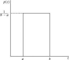
f(x)= 1/(b-a) when a≤x≤b
f(x) = 0 otherwise

Front 38

Probability Density Graph vs Probability Distribution Graph

Back 38

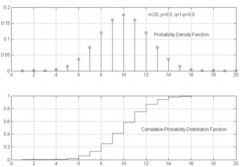
Probability density would look like impulses and probability distribution would look like steps starting at lowest probability and ending at 1

Front 39

Uniform Distribution Function

Back 39

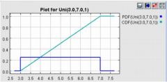
F(x)=∫(1/(b-a)dλ, a, x) =(x-a)/(b-a)

(see green line)

Front 40

Normal (Gaussian)

Back 40

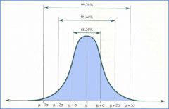
N(μ,σ)

μ=mean=average value
σ^2=variance
σ=standard deviation

Front 41

Standard Normal Probability Density Function

Back 41

N(0,1)

Front 42

Normal Distribution: P(x1<x<x2)

Back 42

F(x2)-F(x1)
=G((x2-μ)/σ)-G((x1-μ)/σ)

(we calculate the value inside, and then use a table to find the values of G(a), G(b), etc)

Front 43

Binomial

another name

Back 43

Bernoulli Trials

Front 44

Binomial

definition

Back 44

Composed of n identical independent trials. Each trial has two outcomes (success p or failure q). The random variable X defines the number of successes in n trials.

Front 45

Binomial density function approximation when we have a large number of trials

Back 45

Can be approximated withth eGaussian density function of N(np, npq)

mean = np
standard deviation = npq

Front 46

Poisson

Back 46

Counts the number of occurrences of an event in a certain time period.

Pk=P(x=k)=e^(-a)*a^k/k!

where a is the average number of event occurances in the same time interval

Front 47

Approximation of binomial

Back 47

large number of trials, small number of successes

we set avg number of event occurances a=np

Front 48

Joint Probability distribution function

Back 48

Fxy(x1,y1)=P((X<=x1)(Y<=y1))

Front 49

marginal distribution of y

Back 49

Fxy(∞,y)=Fy(y)

Front 50

marginal distribution of y

Back 50

Fxy(x,∞)=Fx(x)

Front 51

Joint Density Function

Back 51

F(x,y)=∫(∫(fxy(α,β)dα,-∞,x)dβ,-∞,y)

P((x1<X<x2)(y1<Y<y2))
=∫(∫(fxy(x,y)dx,x1,x2)dy,y1,y2)

Front 52

Independent random variables

Probability
Fxy(x,y)
fxy(x,y)

Back 52

P((X<=x)(Y<=y))=P(X<=x)P(Y<=y)

Fxy(x,y)=Fx(x)Fy(y)
fxy(x,y)=fx(x)fy(y)

Front 53

Conditional Probability Distribution Function

Back 53

F(x|B) is conditional distribution fu of RV x assuming B is defined as the conditional probability of event X<=x

Front 54

Expected Values:

expected value or mean of a function g(x)

Back 54

E[g(x)]=

integral from -inf. to inf. of g(x) * f(x) for continuous

summation of g(xi)P(xi)

Front 55

Mean

Back 55

E[X]=

Front 56

Expected Values

Back 56

E[x]= integral(xf(x)dx)

over the range of -inf to inf

Front 57

Mean

Back 57

E[x]

Front 58

Variance

Back 58

σ^2,

=E[x^2(t)]-E^2[x(t)]

Front 59

Moments

Back 59

m_n=E[x^n]

Front 60

Standard deviation

Back 60

σ, square root of variance

Front 61

Covariance

Back 61

measure of how much two variables change together

If two variables tend to vary together (that is, when one of them is above its expected value, then the other variable tends to be above its expected value too), then the covariance between the two variables will be positive. On the other hand, when one of them is above its expected value the other variable tends to be below its expected value, then the covariance between the two variables will be negative.

Front 62

Covariance

equation

Back 62

Cxy=E[XY]-E[X]E[Y]

Front 63

Correlation

Back 63

E[XY]=Rxy

correlation refers to the departure of two random variables from independence

Front 64

Covariance and Correlation of uncorrelated random variables

Back 64

Covariance = Cxy=0
Correlation=Rxy=E[x]E[y]

Front 65

Orthogonality

Back 65

Correlation = Rxy=0

Front 66

Correlation and Independence

Back 66

Independence will give us uncorrelatedness but not the other way around

Front 67

Characteristic Function

Back 67

the characteristic function of any random variable completely defines its probability distribution.

Front 68

Stochastic Process

Back 68

If a random variable X is a rule for assigning a number X(psi) to every outcome psi of an experiment.

A stochastic process X(t) is a rule for assigning a function X(t,psi) to every outcome psi.

Front 69

Random sequence

Back 69

A random process for which time has only discrete values.

Front 70

Deterministic process

Back 70

Future values of any sample function can be predicted from past values.

Front 71

Non deterministic process

Back 71

Also called regular process. Consists of sample functions that cannot be predicted from past values.

Front 72

Stationary

Back 72

A random process (ie "stochastic process") is stationary if the joint probability distribution does not change when shifted in time or space.

Front 73

Example of stationary process

Back 73

White Noise

Front 74

Properties of a stationary process

Back 74

mean and variance do not change over time (they are constants)

F(x1,x2) depends only on difference between time samples

Autocorrelation Rx(t1,t2)=Rx(t2-t1)

Autocovariance Cx(t1,t2)=Cx(t2-t1)

Front 75

WSS

Back 75

"wide sense stationary" or "weak sense stationary"

only requires the first and second moments to not vary with respect to time (so first and second moments are constant)

Front 76

Conditions to be WSS

Back 76

E(x)=constant

Autocovariance Cx(t1,t2)=Cx(t1-t2) for all t1, t2 (ie depends only on difference between time samples)

(as a result the autocorrelation Rx(t1,t2)=Rx(t2-t1))

Front 77

Properties of WSS

Mean
Variance
Autocovariance
Autocorrelation

Back 77

Mean: constant

Variance: constant (b/c composed of 1st and 2nd moments)

Autocovariance: depends only on difference between time samples

Autocorrelation: depends only on difference between time samples

Front 78

Properties of WSS

Autocorrelation

Back 78

1. Average power (2nd moment) of the process is given at τ=0

R(0)=E[x(t)^2] for all t

2) even fu of τ

Rx(τ)=Rx(-τ)

3) measure of the rate of change of a random process

4) max at τ=0

|Rx(τ)|<=Rx(0)

Front 79

Second order joint distribution

Back 79

F(x1,x2;t1,t2)=P(X(t1)<=x1, X(t2)<=x2))

Front 80

Autocorrelation when t1=t2

Back 80

when t1=t2=t our autocorrelation is equal to the mean squared value (or average power) of X(t)

Front 81

Autocorrelation

Back 81

The autocorrelation of X(t) at two time instants of t1 and t2 is the correlation between two random variables X(t1) and X(t2).

Also known as teh joint moment of X(t1) and X(t2)

Front 82

Uncorrelated

Back 82

Random variables whose cross covariance is zero are called uncorrelated.

Uncorrelated random variables have a correlation coefficient of zero

If X and Y are independent, then they are uncorrelated (but not necessarily the other way around)

Front 83

Covariance

Back 83

E[XY]-E[X]E[Y]

covariance is a measure of how much two variables change together

If two variables tend to vary together (that is, when one of them is above its expected value, then the other variable tends to be above its expected value too), then the covariance between the two variables will be positive. On the other hand, when one of them is above its expected value the other variable tends to be below its expected value, then the covariance between the two variables will be negative.

Front 84

Covariance and Correlation

Back 84

when E[x(t)]=0

Covariance=Correlation

Front 85

Variance vs Covariance

Back 85

variance is a special case of the covariance when the two variables X and Y are identical

Front 86

Orthogonal

Back 86

if the cross correlation Rxy is zero then X and Y are called orthogonal random processes

Front 87

δ(t1-t2)

Back 87

1 when t1=t2
0 otherwise

Front 88

Cross correlation and cross variance

Back 88

used to distinguish from the covariance of a single variable but we loosely use the term covariance for both

Rxy=E[XY]
same as
Rxy(t1,t2)=E[X(t1)Y(t2)]

Cxy=Rxy-E[X]E[Y]
same as
Cxy(t1,t2)=Rxy(t1,t2)-E[X(t1)]E[Y(t2)]

Front 89

How to calculate the autocorrelation

Back 89

∫∫xyf(xy) dxdy, -∞,∞

double integral of the probability density function with respect to the x and y variables from -∞ to ∞

Front 90

impulse response

Back 90

the response of a linear time invariant system to an input unit delta function δ(t) is called the impulse response h(t)

Front 91

causality

Back 91

a system is said to be causal if the response at time t depends only on the present and past values of the input.

Front 92

State Space Representation

Back 92

Dynamic systems are represented by a system of ordinary linear differential equations.

The dependent variables become the state variables.

Any physical system can be represented by the state space representation (which includes a state/plant equation and an output equation)

Front 93

State Variables

Back 93

Dependent variables in a dynamic system represented by a system of linear differential eqns.

The state variables represent all the internal characteristics of the dynamic system.

They cannot generally be measured directly (they are "hidden variables")

Front 94

Input of State Space Eqns

Back 94

u(t)

Properties:

(1) Deterministic: known or measurable by us

(2) Random: known statistical properties such as mean, variance, etc.

Front 95

Output of state space eqns

Back 95

y(t) or z(t)

known through measurements

Front 96

Form of state space equations:

Back 96

x'(t)=Ax(t)+Bu(t)
y'(t)=Cx(t)+Du(t)

OR

x'(t)=F(t)x(t)+C(t)u(t)
z(t)=H(t)x(t)+D(t)u(t)

Front 97

State Equation

(another name)

Back 97

Plant Equation

Front 98

State Equation:

Back 98

State Equation/Plant Equation

x'(t)=F(t)x(t)+C(t)u(t)

F(t) is the dynamic coefficient matrix
C(t) is the input coupling matrix

Front 99

Output Equation

Back 99

z(t)=H(t)x(t)+D(t)u(t)

H(t) is the measurement sensitivity matrix
D(t) is the input/output coupling matrix

Front 100

What can be measured in the state equation

Back 100

only the inputs and outputs of the system can be measured

Front 101

State space representation:

time invariant

Back 101

F(t)=F, H(t)=H, C(t)=C, D(t)=D

x'(t)=Fx(t)+Cu(t)
z(t)=Hx(t)+Du(t)

Front 102

Fundamental Matrix

(another name)

Back 102

State transition matrix

Front 103

State transition matrix

Back 103

State transition matrix, Φ(t)

Transforms the initial state x(t0), of the dynamic system to the corresponding state at time t, x(t)

Front 104

Fundamental matrix

Time invariant system

(equation)

Back 104

Φ(t)=e^(-At)=Laplace((sI-A)^-1)

where A=F

Front 105

Observability

(definition)

Back 105

Observability is the question of whether the states of a given dynamic system are uniquely determinable from it's inputs and outputs, given a model of the system (ie F, H, C, D).

So, given z(t) and the system model, can we find all states (ie x'(t)) of the system.

Front 106

Controllability

(definition)

Back 106

The question is wheter we can, with a given input (or control) go from one state to another state

Front 107

Given:

x'(t)=F(t)x(t)+G(t)w(t)+C(t)u(t)
z(t)=H(t)x(t)+v(t)+D(t)u(t)

what is w(t) and v(t)?

Back 107

w(t): process noise
v(t): sensor or measurement noise

these are usually uncorrelated zero mean processes

E[w(t)]=0
E[v(t)]=0